<?xml version="1.0" encoding="utf-8"?><feed xmlns="http://www.w3.org/2005/Atom" ><generator uri="https://jekyllrb.com/" version="3.10.0">Jekyll</generator><link href="https://evogytis.github.io/feed.xml" rel="self" type="application/atom+xml" /><link href="https://evogytis.github.io/" rel="alternate" type="text/html" /><updated>2026-04-02T08:30:13+03:00</updated><id>https://evogytis.github.io/feed.xml</id><title type="html">Gytis Dudas</title><subtitle>personal website</subtitle><author><name>Gytis Dudas</name><email>gytis.dudas@gmc.vu.lt</email></author><entry><title type="html">Part 1: the paper with eight segments and eight co-first authors</title><link href="https://evogytis.github.io/posts/2024/02/batson-california/" rel="alternate" type="text/html" title="Part 1: the paper with eight segments and eight co-first authors" /><published>2024-02-19T00:00:00+02:00</published><updated>2024-02-19T00:00:00+02:00</updated><id>https://evogytis.github.io/posts/2024/02/batson</id><content type="html" xml:base="https://evogytis.github.io/posts/2024/02/batson-california/"><![CDATA[<h2 id="background">Background</h2>

<p>As mentioned in the <a href="https://evogytis.github.io/posts/2024/02/metagenomics/">introductory post</a> this is the blog post about the <a href="https://elifesciences.org/articles/68353">Batson <em>et al.</em> (2021)</a> study that started it all. When I joined Biohub remotely in late 2018 the California mosquito transcriptomes were still quite fresh but what do we do with these data? The main question that these pilot data were meant to be addressing - whether we can find viruses relevant to human health in mosquitoes prior to human cases - was clearly a “no”. What do we do now then? I spent much of 2018 and early 2019 probing these data and discussing potential avenues of research with the Biohub team - almost always Amy Kistler, Joshua Batson, Hanna Retallack, Lucy Li, and Kalani Ratnasiri - over evening Zoom calls (thanks to unfortunate differences between European and US West Coast timezones). Mind you these were pre-pandemic Zoom meetings, <em>i.e.</em> before it was cool. As usual, here’s the story of how the paper came about (from my perspective).</p>

<h2 id="the-power-of-repeating-repeating-repeating">The power of repeating repeating repeating</h2>

<p>As expected, and as will be discussed in another blog post, the more people focus on sequencing particular groups of hosts, the more likely they are to dredge up similar viruses. Though undeniably vast, virus diversity is finite after all. That does not mean that every project setting out to discover new viruses should be disappointed when previously described viruses are found. I think these cases help us out in two ways - first, multiple detections of the same genetic material acts as <a href="https://en.wikipedia.org/wiki/Repetition_code">repetition code repetition code</a>, an error correction method in coding theory where transmission of a message over a noisy channel achieves fidelity by repeating the message. Let’s say you assembled a contig with two completely overlapping ORFs running in opposite directions - was that a statistical fluke? It becomes difficult to argue that it is if someone else saw that before and even more so if your data has 40-odd contigs that look that way. Likewise for ORF positions, likewise contig ends, assembly artefacts, <em>etc</em>.</p>

<p>The second thing repeated detections of the same virus can do is something I’ve dreamed of for a while. Here’s the problem - your <em>de novo</em> assembled contigs from a metagenomic sequencing run is contig soup. Typically you’ll determine what’s what by sequence similarity to something that’s already known on public databases. If you have an RNA virus with an unsegmented genome you’re sorted - genes B, C, and D are clearly viral in origin even if they don’t resemble anything out there if they’re on the same piece of RNA with gene A that is a conserved virus gene that has annotated relatives. But good luck recognising this if genes B, C, and D are on separate segments of a segmented genome - they’re metagenomic “dark matter” now, genetic material you’d like to know about but cannot. There’s two approaches you can take here these days. If you work on a host that uses RNAi as its defense (like an arthropod) you can use small interfering RNA (siRNA) sequencing since those siRNAs will have been generated from double-stranded RNA (dsRNA) that was inside the cell and got caught. When not being used to regulate gene expression, dsRNA is also a dead giveaway of a replicating RNA virus so if you see siRNA reads aligning to your contigs it means your arthropod thought those contigs existed as dsRNA inside the cell and are strong virus candidates. Galbut (technically Galbūt) and Chaq viruses were <a href="https://journals.plos.org/plosbiology/article?id=10.1371/journal.pbio.1002210">discovered in this way</a> by Darren Obbard and both names indicate uncertainty in Lithuanian and Klingon, respectively (two fictional languages, per Darren’s jest), since it was not 100% guaranteed they were actually viruses.</p>

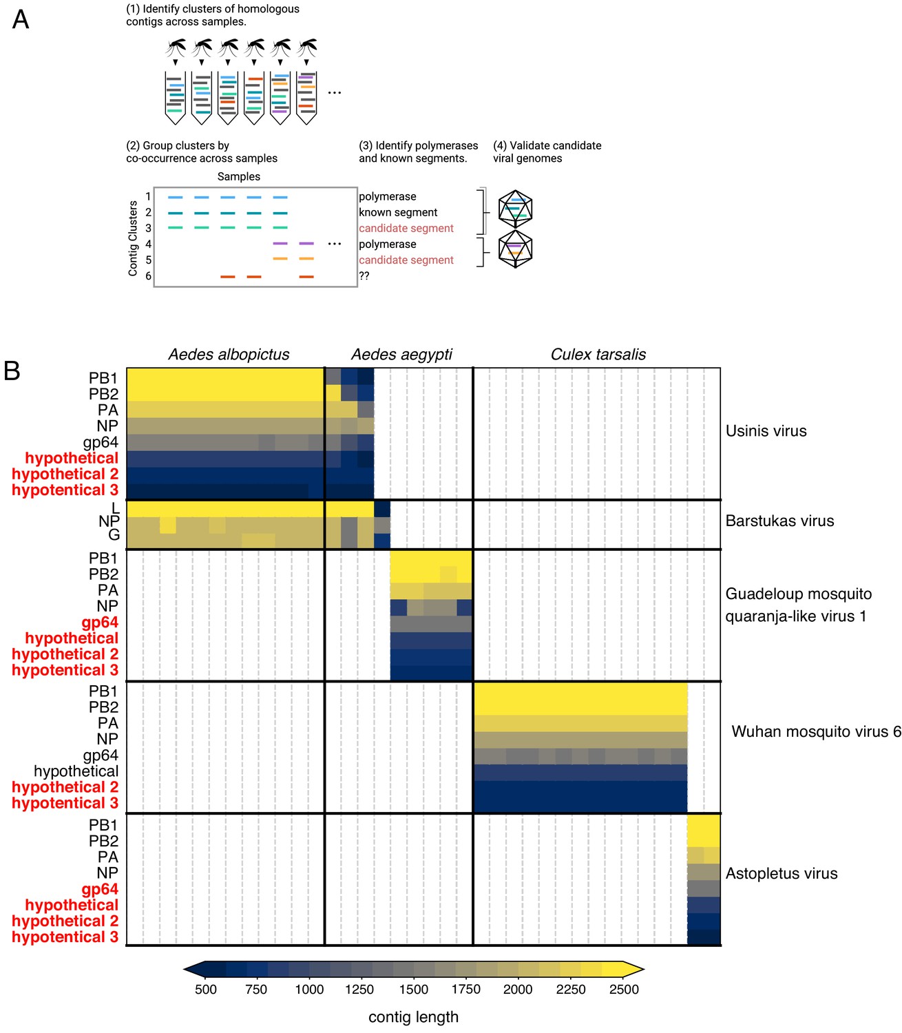
<p>The other method for detecting likely viral sequences is simpler and gains power with each new dataset and relies on co-occurrence. Darren Obbard used this method to identify <a href="https://academic.oup.com/ve/article/6/1/vez061/5708932">an entirely new family of RNA viruses</a> in August 2019 and funnily enough Joshua Batson was writing code to do <a href="https://github.com/czbiohub-sf/california-mosquito-study/blob/0ff3089300111459cd295b019f54a3c36a41fca3/notebooks/Multisegmented%20Virus%20Hunting.ipynb">exactly the same thing around the same time</a>. Back in January 2019 when presenting to the rest of the team I highlighted two viruses - Wuhan mosquito virus 6 (WuMV-6, an orthomyxo) and Culex narnavirus 1 (CxNV-1, a narna). WuMV-6 caught my attention because it was an orthomyxovirus that was seen before and quite common in our data while CxNV-1 had the unusual property of being ambigrammatic (having two completely overlapping ORFs running in opposite directions). In those January 2019 slides I put a rhetorical “fish out the rest of the genome?” near some early four segment (the most conserved PB1, PB2, PA, and NP) WuMV-6 phylogenies. When I took Josh’s code for a spin on our data my mind was immediately blown. By that point we already knew from <a href="https://jvi.asm.org/content/91/17/e00680-17">Mang Shi and Eddie Holmes’ work</a> that WuMV-6 had at least six segments but Josh’s code found another two. Obviously, they don’t resemble anything on GenBank and so could never be fished out of the contig soup by sequence similarity before but could be now - especially from other people’s data which convinced us we were seeing genuine segments. By the way - Culex narnavirus 1 turned out to have a previously unrecognised segment. Also ambigrammatic but more on that in <a href="https://evogytis.github.io/posts/2024/02/dudas/">a sister blog post</a>.</p>

<p><img src="https://iiif.elifesciences.org/lax/68353%2Felife-68353-fig6-v2.tif/full/,1500/0/default.jpg" alt="Segment co-occurrence" /></p>

<h2 id="what-now-organise-re-organise">What now? Organise, re-organise</h2>

<p>Armed with Josh’s new contig co-occurrence detection code Josh I realised we had to organise the viral portion of our data in a way that made sense moving forwards. Before we were relying on similarity (BLAST hits) to identify viral sequences and pull them out individually for other kinds of analyses (<em>e.g.</em> phylogenetics) or using BLAST results to look at the taxonomic breakdown of read counts. This wasn’t at all helpful in adding the metagenomic “dark matter” we pulled into the light with Josh’s code nor helpful in eventually submitting these sequences to GenBank. Josh’s code was quite helpful in another way - <a href="https://www.cell.com/current-biology/fulltext/S0960-9822(17)31267-8">arthropod genomes can contain endogenous viral elements (EVEs) that are actually expressed as RNA</a> so even if you identify a clearly viral contig in your transcriptome it’s not always guaranteed to be from a virus that’s there right now. We definitely had a few (-)ssRNA NP sequences hanging out in a few samples on their own nor co-occurring with anything else across multiple samples. Since arthropod EVEs (endogenous viral elements) are thought to come from viral mRNAs (where common transcripts are more likely to integrate) and since we were going to have to screen all of our contigs for co-occurrence, I reorganised all of our viral data based on RNA-dependent RNA polymerases (RdRps) since that’s a core requirement for an autonomous RNA virus and one of the rarer transcripts during infection that’s less likely to end up as an EVE. First we used hidden Markov models (HMMs) to fish out RdRps from our data then we used the RdRps as baits in Josh’s code to find the rest of the genome if it was segmented.</p>

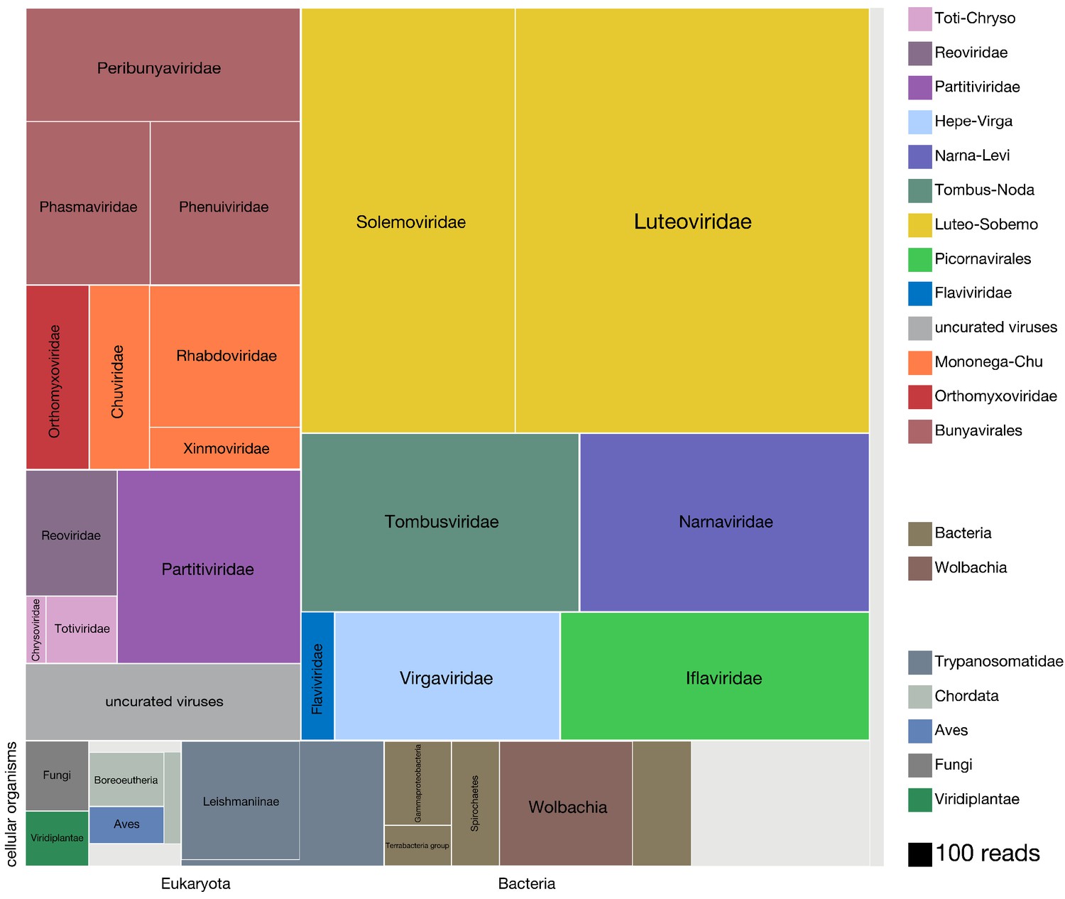
<p>Over the course of this project another less pleasant reorganisation was happening on GenBank. Relatively early in my work on the <a href="https://iiif.elifesciences.org/lax/68353%2Felife-68353-fig2-v2.tif/full/1500,/0/default.jpg">treemap figure</a> NCBI’s virus taxonomy (which I was using to organise the treemap compartments) suddenly changed to reflect <a href="https://journals.asm.org/doi/10.1128/mbio.02329-18">one proposed alternative system</a>, despite some <a href="https://journals.asm.org/doi/10.1128/mbio.00289-19">very serious issues brought up about its methodology</a>. In my opinion taxonomy is a fun little exercise that’s not to be taken too seriously since it’s subjective. On occasion virus taxonomy has made sense - <em>Orthomyxoviridae</em>, being a clade of (-)ssRNA viruses that use a heterotrimeric RdRp, and code for NP, at least one surface protein, and something to form a matrix, make sense as a taxonomic grouping, I’ll go as far as saying that the taxonomic rank of family might be useful for classifying viruses. However, in its current state virus taxonomy is peppered with ridiculous (read: over-split) and hypothetical (read: ambitious, given the divergence) taxonomic ranks that, if ever confirmed by research in the coming decades, I suspect will have been arrived at by chance. Annoyingly, following the transition to the new taxonomy I had viruses sitting both in the new (apparently) phylum <em>Negarnaviricota</em> (I’m fine with this since (-)ssRNA viruses are distinctly related) and the old “ssRNA negative-strand viruses”. Far from ideal. I guess the lesson from this little detour is that sometimes there will be people who care about something even if you don’t, so if you rely on things others have a say in you might be in for an unpleasant surprise down the line.</p>

<h2 id="is-it-really-a-segment">Is it really a segment?</h2>

<p>Using Josh’s co-occurrence method I was able to identify a total 15 novel segments associated with six viral RdRps and add more weight to the developing thought that Darren’s Chaq “virus” is actually a satellite segment of (also Darren’s) Galbut virus by observing co-occurrence of sequences related to both Chaq and Galbut (called Nefer virus in our data). Most (13) of the novel (<em>i.e.</em> unBLASTable) segments we identified belonged to orthomyxos - some were highly diverged surface proteins gp64 (but recognisable as such by HMM), and the rest (with the exception of WuMV-6 hypothetical segment discovered previously) were three small segments. It’s not surprising that we found the most new segments for orthomyxos since they have the highest recorded segment number amongst (-)ssRNA viruses and I’m convinced we missed segments of a couple of reoviruses in our data too (for the same reason).</p>

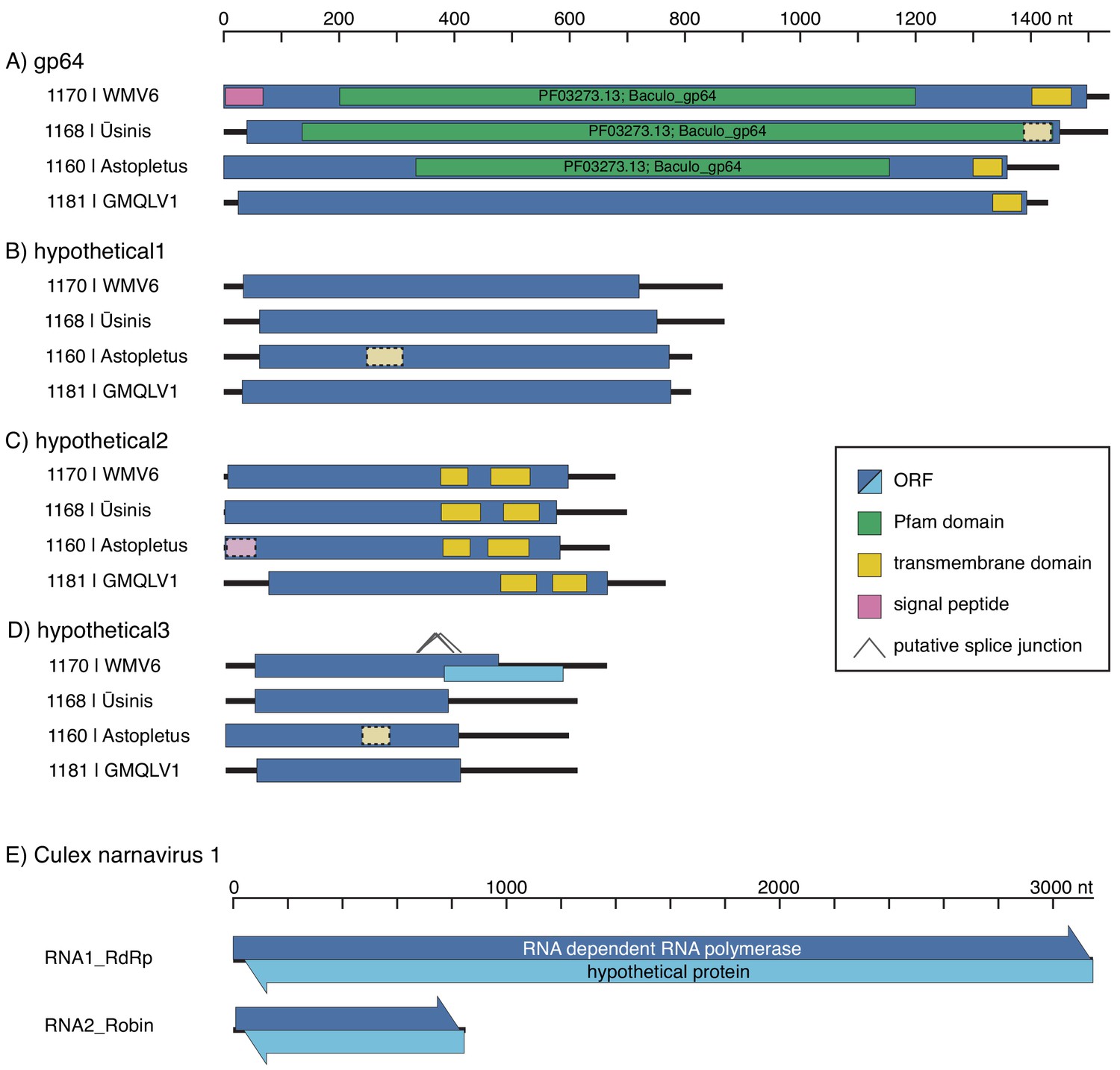
<p><img src="https://iiif.elifesciences.org/lax/68353%2Felife-68353-fig6-figsupp2-v2.tif/full/1500,/0/default.jpg" alt="Similar features of otherwise unrecognisably related segments" /></p>

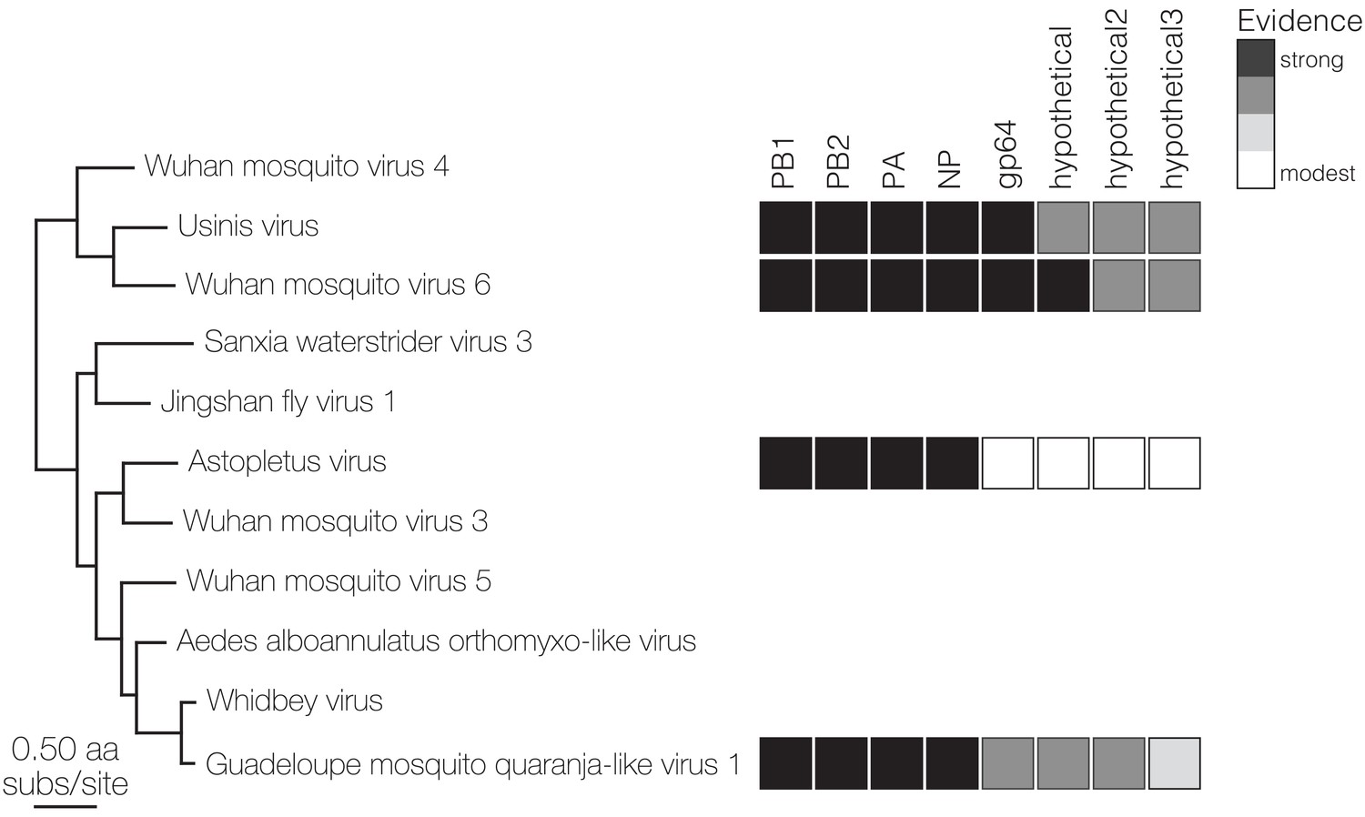
<p>As we quickly discovered we couldn’t delve very deep into the new orthomyxo segments we found since not only did they not resemble anything on GenBank at that point but they didn’t even look like <em>each other</em>. Being the scientists that we are we therefore had to convince ourselves these segments were genuine and this was made quite easy: 1) putatively homologous segments shared features - length, transmembrane domains and their number in the case of segment hypothetical 2 or the longest ORF not occupying the full length of the segment and therefore likely to undergo splicing for segment hypothetical 3, 2) the phylogenetic trees we made for all segments of WuMV-6 were quite concordant across putative segments, and 3) we could either assemble all of the missing segments from other people’s data (for WuMV-6 and Guadeloupe mosquito-associated quaranjavirus 1) or saw reads that upon translation looked like they could be related, basically strong evidence that a broader clade of orthomyxos had this eight segment genome organisation. In my opinion, the ability to reconstruct these segments from other people’s data makes it conclusive and it’s very nice to see a proliferation of tools targeting the vast mountain of data sitting on NCBI’s sequence read archive (SRA) that help immensely with this task. <a href="https://www.biorxiv.org/content/10.1101/2023.07.09.547343v1">Pebblescount</a> and <a href="https://www.nature.com/articles/s41586-021-04332-2">Serratus</a> are the ones I know/use most, by the way.</p>

<p><img src="https://iiif.elifesciences.org/lax/68353%2Felife-68353-fig6-figsupp3-v2.tif/full/1500,/0/default.jpg" alt="Convincing evidence for segments" /></p>

<p>The appearance of these tools is also a sign that many crews running sequencing experiments out there aren’t squeezing <em>everything</em> out of their raw data and why should they? Sequencing is ever cheaper and scientific questions motivating the sequencing are not always to do with virus discovery. Having said that, when reads come from virus discovery studies but only the most conserved / easiest to recognise contigs from segmented virus groups are submitted to GenBank I get a bit miffed. RdRps in their ever bewildering forms are extremely informative about RNA virus evolution but the rest of the genome is important too. Surface proteins come to mind here since something that’s receptor binding can (theoretically) make the difference between a virus that’s <a href="https://en.wikipedia.org/wiki/Subtypes_of_HIV#HIV-1">bloodborne</a> or <a href="https://en.wikipedia.org/wiki/Jaagsiekte_sheep_retrovirus">airborne</a> or a virus that’s infecting <a href="https://en.wikipedia.org/wiki/Rift_Valley_fever">you</a> or a <a href="https://en.wikipedia.org/wiki/Leishbunyaviridae"><em>Trypanosome</em></a> inside you. Obviously I’m more than happy to sort through the scraps if it means we’ll understand orthomyxo genome evolution a bit better and at the end of the day having mountains of sequence data that’s not been completely wrung out means there’s an enrichment of the research ecosystem for everyone else, particularly in resource-limited settings.</p>

<h2 id="fascinating-virus-ecology">Fascinating virus ecology</h2>

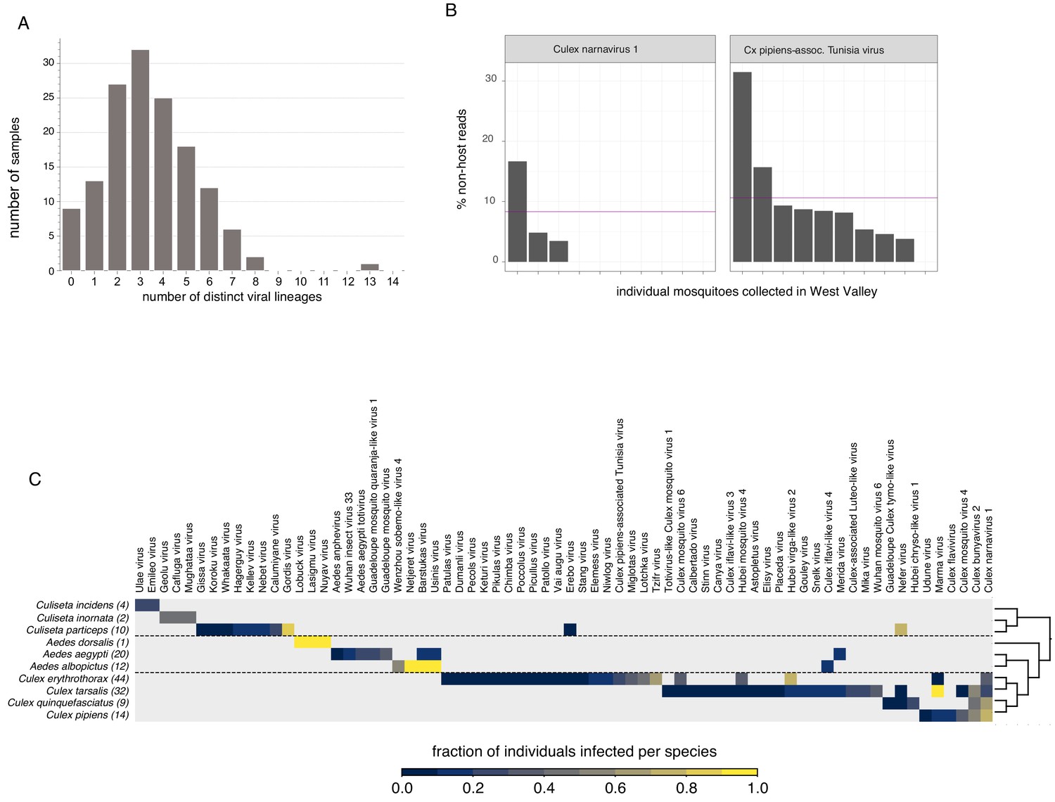
<p>Finally, there’s a couple of very interesting ways we broke down the distribution of viruses found in individual Californian mosquitoes. One obvious breakdown is to look at co-infection - how many distinct viruses do all of our sampled mosquitoes carry simultaneously? What does that histogram look like? We actually had nine mosquitoes without any viruses and one that had 13, the mode was three. The extremes were very telling too - samples without any viruses had low numbers of reads overall (so probably low quality) while six of the 13 viruses in the unfortunate mosquito were botourmiaviruses (<a href="https://en.wikipedia.org/wiki/Botourmiaviridae">thought to infect fungi</a>) and probably came from the ergot fungus whose reads we also saw in the sample. The inability to determine the host of a given virus in metagenomic data is a known issue with some tools to address it (<em>e.g.</em> siRNA sequencing mentioned earlier) though I suspect with ever increasing amounts of sequence data we’ll come to rely more and more on the phylogenetic signal of certain virus groups associating with certain host groups as a useful proxy.</p>

<p><img src="https://iiif.elifesciences.org/lax/68353%2Felife-68353-fig4-v2.tif/full/1500,/0/default.jpg" alt="Co-infection and host tropism" /></p>

<p>The next bit surprised me and I’m still not sure if it should have or not. At one point we decided to look at the distribution of viruses we found per mosquito species (bottom heatmap). Somewhat surprisingly, most of our viruses looked like they were very species-specific, <em>e.g.</em> Ūsinis is overwhelmingly found in <em>Aedes albopictus</em> (I suspect its presence in <em>Aedes aegypti</em> might be contamination) while Wuhan mosquito virus 6 (its closest relative) is found in <em>Culex tarsalis</em>. Having assembled numerous WuMV-6 genomes from SRAs it’s clear that WuMV-6 can also infect <em>Culex quinquefasciatus</em>, <em>Cx. pipiens</em>, <em>Cx. australicus</em>, and <em>Cx. globocoxitus</em> (<em>Haemagogus</em>, a member of <em>Aedini</em> too, allegedly). So on one hand we have a virus that’s not terribly picky about hosts as long as their Latin binomial starts with <em>Culex</em> but on the other hand we found it solely in <em>Cx. tarsalis</em> in California even though other hosts were available. This implies some sort of dynamics that we won’t be able to disentangle until we have more WuMV-6 genomes collected more consistently in time and space. The poor virome overlap between species also for the time being implies that many viruses might not be suitable for reconstructing community interaction networks because of sparseness.</p>

<h2 id="in-the-shadow-of-the-pandemic">In the shadow of the pandemic</h2>

<p>Picture this timeline: in late 2017 the individual Californian mosquito transcriptomes are sequenced, in late 2018 I join the project, then in late 2019 I’m in SF and we’re finalising the manuscript until suddenly in early 2020 the SARS-CoV-2 pandemic begins. By this point we have a manuscript together. It’s a bit all over the place but there’s just that much interesting stuff in the sequences so we submit it to a journal as is. We get desk rejected, mostly because the manuscript isn’t focused enough but the editor adds insult to injury. In their opinion us highlighting <em>Wuhan</em> mosquito virus 6, a virus unrelated to the SARS-CoV-2 pandemic is <em>inappropriate</em>. That would be a fair comment if we didn’t have Github commits specifically mentioning WuMV-6 going back a year, <em>i.e.</em> before Wuhan was a household name. Unfortunately, this wasn’t the last or the most serious way the pandemic messed with this paper.</p>

<p>CZ Biohub and my co-authors ended up getting heavily involved in California’s SARS-CoV-2 surveillance efforts and that rejection in early 2020 meant that no one had any more time to revisit the manuscript until late 2020. Scrounging what little time we had between ourselves (and overwhelmingly thanks to Amy Kistler) we had a reworked draft ready in December 2020 and we decided to try out <a href="https://www.reviewcommons.org/">Review Commons</a> which is basically outsourced peer review (and why not, reviewers aren’t being paid anyway). (Many things were happening then - the other two papers that I’ll discuss in sister posts <a href="https://evogytis.github.io/posts/2024/02/dudas/">A</a> and <a href="https://evogytis.github.io/posts/2024/02/dudas-batson/">B</a> were born during this time, as well as <a href="https://evogytis.github.io/posts/2021/10/B1620/">Lithuania’s SARS-CoV-2 genomic surveillance programme</a>.) We had the reviews from Review Commons back by February 2021 which were mostly positive so after another month of working on the comments during the precious hours between the mountain of work that was COVID-19 we sent the revised manuscript back to Review Commons. With the reviewers’ final approval we then had to decide which journal to submit to. Since we had positive reviews and a largely overhauled manuscript, I pushed Amy to submit to the same journal that desk-rejected us a year ago and to our surprise it got accepted! The rest is history.</p>

<h2 id="what-of-all-this">What of all this?</h2>

<p>To this day the individual California mosquito metatranscriptome project remains my favourite for many reasons. First and foremost, I got a chance to meet and work together with knowledgeable and lovely people (special shout out here to Joshua Batson, Amy Kistler, Lucy Lu, and Hanna Retallack) as a domain expert and working with experts from other domains. Don’t get me wrong, working on large genomic epidemiology studies was fun but it’s quite difficult to shine when everyone in the room has largely the same expertise as you.</p>

<p>Working on this study was also very rewarding because it allowed to make significant contributions to the orthomyxovirus field - fishing out novel segments that don’t resemble anything at all was a dream of mine for a long time. To be fair just working in metagenomics and virus discovery was a dream too. Finally, I have to thank this study for where I am today - by finding Wuhan mosquito virus 6 and the broader clade it belongs to I had a promising study system - not only accessible (WuMV-6 really does look like it’s everywhere) but also interesting in many fascinating ways. <a href="https://www.embo.org/people/investigating-virus-ecology-and-evolution/">EMBO thought so too</a>, we even <a href="https://www.embo.org/podcasts/its-viruses-all-the-way-down-a-conversation-with-hsiao-han-chang-gytis-dudas-and-hedvig-tamman/">talked a bit about it recently</a>. Five years after joining a Zoom call with unfamiliar people sitting in San Francisco, today those people are still my friends and colleagues, I have more confidence in my abilities (<a href="https://evogytis.github.io/posts/2021/10/B1620/">see a theme?</a>), and this whole academia thing seems like it’s going as well as it can.</p>]]></content><author><name>Gytis Dudas</name><email>gytis.dudas@gmc.vu.lt</email></author><category term="metagenomics" /><category term="virus discovery" /><category term="orthomyxos" /><category term="WuMV-6" /><summary type="html"><![CDATA[Background]]></summary></entry><entry><title type="html">Part 3: the paper with Wuhan mosquito virus 6 and Josh</title><link href="https://evogytis.github.io/posts/2024/02/dudas-batson/" rel="alternate" type="text/html" title="Part 3: the paper with Wuhan mosquito virus 6 and Josh" /><published>2024-02-19T00:00:00+02:00</published><updated>2024-02-19T00:00:00+02:00</updated><id>https://evogytis.github.io/posts/2024/02/dudas-batson</id><content type="html" xml:base="https://evogytis.github.io/posts/2024/02/dudas-batson/"><![CDATA[<p>If you’re going in chronological order you’ve already read about how I got involved with Chan Zuckerberg’s Biohub <a href="https://elifesciences.org/articles/68353">individual mosquito transcriptome project</a>, the exciting findings <a href="https://evogytis.github.io/posts/2024/02/batson-california/">from it and the issues it faced</a>, a brief foray into <a href="https://evogytis.github.io/posts/2024/02/dudas/">collaboration on one of the interesting viruses we stumbled upon</a>, and now I’ll tell you about <a href="https://journals.asm.org/doi/10.1128/jvi.01056-23">the most recent paper</a> that came out of the Californian mosquito data. It’s both a kind of love story and a mission statement for my lab as we go forward.</p>

<h2 id="background">Background</h2>

<p>Picture this - as we’re wrapping up and polishing the main individual Californian mosquito transcriptome paper a number of analyses that I had done remain overboard. Many of them are from a time when we thought of the paper as being a compilation of vignettes - short self-contained stories highlighting some interesting aspect of virus biology that was enabled by our study design. Some I’m keeping for potential metagenomically-inclined PhD students, others were not that exciting in retrospect, and the rest I’ll talk about here.</p>

<p>I should also say that this particular study lingered on my desk an unbelievably long time. I had an early draft of this paper in late 2020 with a slightly different framing that was marinating until 2022 when Josh and I mustered enough motivation to push through the last round of revisions for it. After that we put it up on <a href="https://www.biorxiv.org/content/10.1101/2022.08.31.505987v4.article-info">bioRxiv</a> and initially sent it to <a href="https://www.reviewcommons.org/">Review Commons</a> for peer review (try it if you haven’t!). I was very pleasantly surprised when an editor of <a href="https://academic.oup.com/evlett">Evolution Letters</a> reached out to see if we wanted to submit it there but unfortunately we had other plans in mind. Since Journal of Virology doesn’t recognise reviews from Review Commons we had to do more rounds of peer review which was fine by me, we even got some <a href="https://journals.asm.org/doi/10.1128/jvi.01056-23#supplementary-materials">solid confirmation</a> that we weren’t getting the interesting results because of some fluke.</p>

<p>Before I go into any of the details I feel like I should give you one crucial piece of information to understand why I did this study the way I did it. I love orthomyxos (members of <em>Orthomyxoviridae</em>). Have since my early PhD days. It’s what my first first-author paper is on. I love that its diversity is amenable to family-wide analyses, love the genome organisation, love its tractable reassortant way of recombining, and I certainly appreciate that its members can be a problem for vertebrate health.</p>

<h2 id="the-vignette">The vignette</h2>

<p>One of the first things that was left overboard with the Batson <em>et al</em>. (2021) paper was a reassortment network of Wuhan mosquito virus 6 (WuMV-6). The paper felt busy as it is without an arbitrary deeper dive into an obscure virus. We already had all the orthomyxo finds we could want - <a href="https://elifesciences.org/articles/68353/figures#fig6">an eight-segmented clade</a>, <a href="https://elifesciences.org/articles/68353/figures#fig6s3">reconstruction of putative segments from other people’s data</a>, <a href="https://elifesciences.org/articles/68353/figures#fig7">some phylogenetics showing expected patterns of diversity and some reassortment</a>. A deeper dive into WuMV-6 would’ve detracted from the paper whilst not doing our finding any justice. It was agreed that I was free to pursue the story on my own.</p>

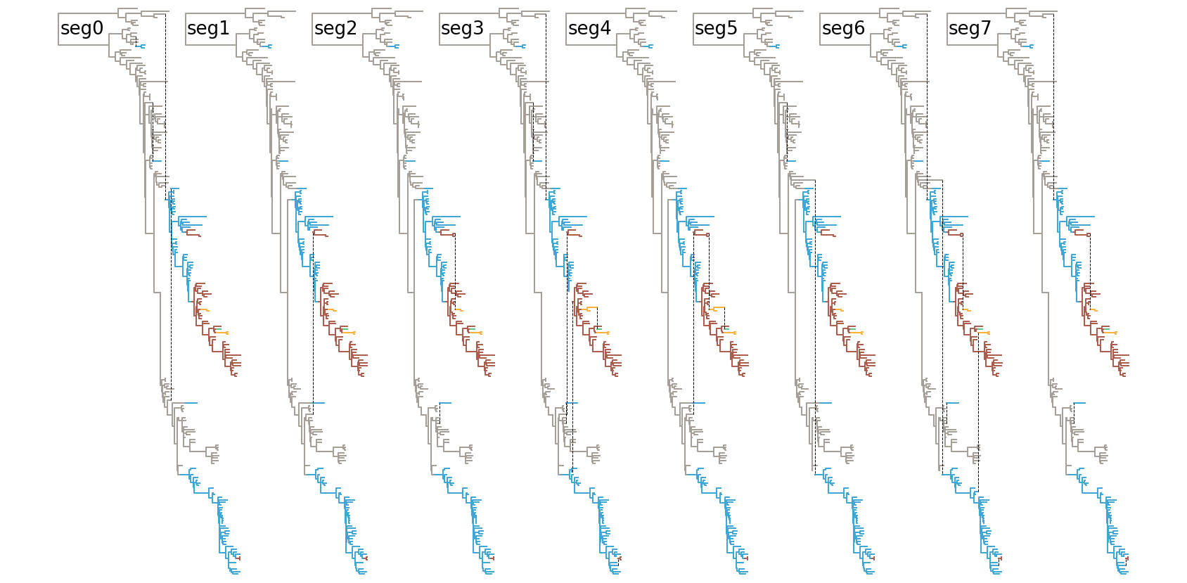
<p>As I was working through some early analyses with WuMV-6 genomes from <a href="https://elifesciences.org/articles/05378">China</a>, <a href="https://elifesciences.org/articles/68353">California</a>, and <a href="https://journals.asm.org/doi/10.1128/jvi.00680-17">Australia</a> more WuMV-6 sequences started showing up. First in <a href="https://www.mdpi.com/1999-4915/11/11/1033">Sweden</a>, then a collaborator working on mosquitoes in Cambodia found it in their sequence data. This pattern would continue over the years and today we know WuMV-6 is present as far as Trinidad, Tunisia, Madagascar, <em>etc</em>. Such volumes of data collected over time, particularly when segmented (<a href="https://www.pnas.org/doi/abs/10.1073/pnas.1918304117">now that we have the right method to analyse them</a>), are prime targets for analyses in BEAST. Surprisingly enough (since not every RNA virus works in this regard) WuMV-6 genomes showed sufficient molecular clock signal to be calibrated with minimally informative priors and we had our very own 27-genome reassortment network.</p>

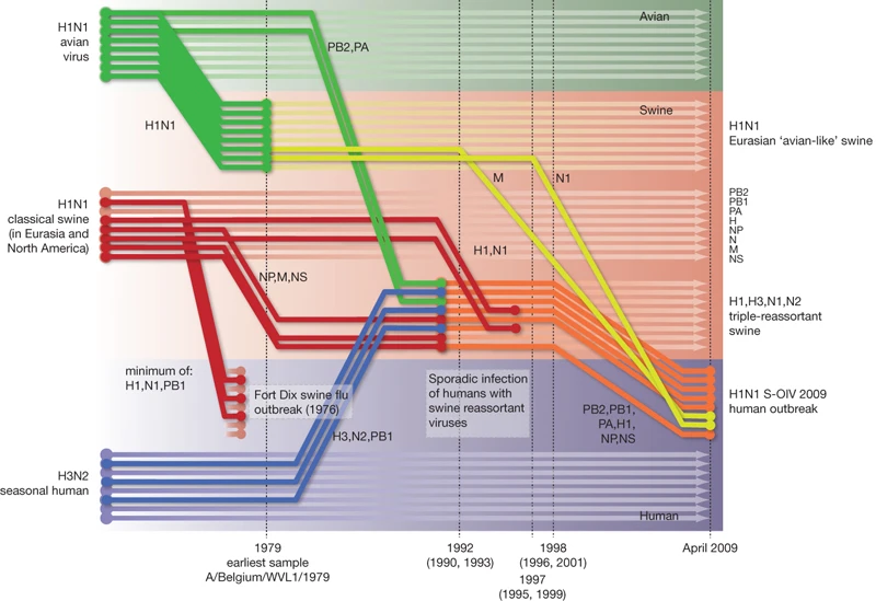
<p>Something that immediately caught my eye is how recent the common ancestry of WuMV-6 genomes was. If you look at WuMV-6 diversity outside of Sweden (which shares a common ancestor with the rest in ~1950s) all of it derives from a single genome that existed in the last ~20 years despite its descendants now being found around the perimeter of the Pacific Ocean - California, China, Cambodia, Australia. Furthermore, we can see reassortment events taking place in the last ~8 years involving lineages that are later found in Australia and California, <em>i.e.</em> opposite sides of the Pacific Ocean. Remarkable rates of migration! But are they really?</p>

<p><img src="https://journals.asm.org/cms/10.1128/jvi.01056-23/asset/f65cb480-ed5d-4aab-827c-72be848ea8d3/assets/images/large/jvi.01056-23.f001.jpg" alt="Did I mention reassortment networks are cool?" /></p>

<p>I think it’s entirely fair to say that we know very little about the lives of insects. We can make many unusual observations - Sigmaviruses in <em>Drosophila</em> being exclusively vertically transmitting yet somehow jumping from <a href="https://journals.plos.org/plosbiology/article?id=10.1371/journal.pbio.1002210">one species to another in the last couple of hundred years</a>, Sigmaviruses <a href="https://royalsocietypublishing.org/doi/full/10.1098/rspb.2012.1208">sweeping in UK</a> on the order of decades, <a href="https://academic.oup.com/mbe/article/5/3/252/972348">the classic global P element (a transposable element) sweep in <em>Drosophila melanogaster</em> that took less than 50 years</a>, (as I’ve recently learned from Darren Obbard on a recent visit) <a href="https://www.pnas.org/doi/full/10.1073/pnas.1500758112">a P element invasion of <em>Drosophila simulans</em> that took a few years to establish it globally but not yet fixed in all populations</a>. We have the observations of a whole spectrum of migration rates (often involving vertical transmission), they’re unambiguous, and yet very little understanding of how those migrations occur. With this little caveat in mind we can proceed to some hypotheses of WuMV-6 migration.</p>

<h2 id="ships-winds-or-meaty-spaceships">Ships, winds, or meaty spaceships?</h2>

<p>It’s common knowledge in arbovirology that mosquitoes are not travelers. They’ll at most travel a few kilometres in their short lives. We’ll set aside the speed with which the vertically-inherited P element invaded <em>Drosophila simulans</em> (also not a strong flier) and look for alternative ways for mosquitoes to go far and fast. Humans have very efficient technological means to go <a href="https://onlinelibrary.wiley.com/doi/full/10.1111/mec.12925?casa_token=Ihdbh7lJeyIAAAAA%3AGfjgk2h16nfl4VyGBfvgY57MqzHcf4wfY4O-cFil6RTLyuS2lHgmvbCz0-Y6CrbxnR2Ucu2KF-b17hDf">far and fast</a>. We also know that mosquitoes can get swept up into the atmosphere where they can <a href="https://www.nature.com/articles/s41586-019-1622-4">ride high altitude winds</a> and get deposited hundreds of kilometres away. And then there’s the classic arbovirus method of travel - inside meaty spaceships called vertebrates. We’ve seen it with <a href="https://www.science.org/doi/full/10.1126/science.aaf5036">Zika over the last 50 years</a> and we’ve seen it with <a href="https://www.pnas.org/doi/full/10.1073/pnas.1206598109">West Nile invading North America in 1999</a>.</p>

<p>We need an extra puzzle piece from WuMV-6 to answer this so I looked into segment-wide dN/dS. I was initially dismayed that segments hypothetical 3 and 2 (unknown function) showed higher segment-wide dN/dS than gp64 (the surface protein). My initial hypothesis was that if WuMV-6 is infecting vertebrates we might see some evidence of antigenic drift that would manifest in a higher dN/dS or higher rates of non-synonymous evolution (seeing as time is a more sensitive way of normalising than more mutations). This was a bit too single-minded of me and it turns out that an analogous situation occurs in influenza - the NS segment - similarly short - <a href="https://www.sciencedirect.com/science/article/pii/S1567134823000229">evolves much faster at the non-synonymous level</a> than haemagglutinin (HA) which we know experiences antigenic drift. In light of this I changed my interpretation of the results - WuMV-6 surface protein gp64 distinctly experiences very high rates of non-synonymous evolution outside the normal range seen in its other longer proteins. Neither anthropogenic transportation methods nor abiotic factors like high altitude winds could explain this pattern but the involvement of vertebrate hosts exherting antibody pressure certainly could. So my current suspicion is that WuMV-6 does infect a somewhat longer-lived vertebrate host with some regularity. It’s almost certainly not humans given that we probably into contact with WuMV-6 all the time but water birds, <a href="https://journals.asm.org/doi/10.1128/jvi.02019-14">already susceptible to other quaranjavirus infections</a>, could be good candidates.</p>

<p><img src="https://journals.asm.org/cms/10.1128/jvi.01056-23/asset/7336aa76-4b26-44e1-92e4-25a9e3097534/assets/images/large/jvi.01056-23.f002.jpg" alt="Surface proteins and non-synonymous evolution" /></p>

<h2 id="a-tale-of-two-classes-of-proteins">A tale of two (classes) of proteins</h2>

<p>One of the goals that I set out for a paper was to have a kind of roadmap figure for orthomyxoviruses. What is the current state of their diversity? How many genomes are complete? What can we say about their surface proteins? What patterns emerge when we synthesise data across studies?</p>

<p>A few things we found:</p>
<ol>
  <li><em>Most orthomyxovirus genomes are incomplete</em>. Public sequence databases are rife with PB1, PB2, PA, and NP because they’re quite conserved and thus easiest to identify by a simple homology search. Without individual-animal metagenomic study designs it’ll take us a lot longer to reconstruct complete genomes and thus to identify and characterise potentially problematic viruses.</li>
  <li><em>Most orthomyxoviruses use one of two membrane fusion protein classes if not actual proteins</em>. Currently known orthomyxoviruses seem to use just one of two membrane fusion protein classes - class I (the haemagglutinins, haemagglutinin-esterase-fusion proteins, and the like) found in vertebrate-infecting members and class III (gp64-like proteins) in predominantly invertebrate-infecting members. That’s an interesting limitation if it’s real. It also comes with curious exceptions - there’s a clade of recently discovered fishy orthomyxos (Steelhead trout orthomyxovirus-1 and Rainbow trout orthomyxovirus-2) that have a recognisable neuraminidase that’s not accompanied by a haemagglutinin which brings us to the next observation.</li>
  <li><em>Too many orthomyxoviruses have mislabeled genes</em>. Despite distinctly not having <em>haemagglutinins</em> both the fishy clade and a number of quaranja- and thogotoviruses are labeled as such. All currently known thogoto- and quaranjaviruses use gp64 proteins (class III) and the fishy clade seems to be using another unrelated (or unrecognisably related) class I protein that seems closer to SARS-CoV-2 Spike or retroviral <em>env</em>. I blame this on the familiarity with influenza A as the archetypal orthomyxovirus (so anything that’s a surface protein gets called haemagglutinin) and the lack of curation on public databases.</li>
</ol>

<p>All of these point to our ability to do better as the research community.</p>

<h2 id="are-we-there-yet">Are we there yet?</h2>

<p>RNA virus diversity is finite. Yes, it is vast but also has to be finite. Because of the way phylogenetics works whenever we discover a new sequence we also get to know a bit about their evolutionary history too. With <a href="https://www.biorxiv.org/content/10.1101/2023.04.18.537342v1">some exceptions</a> it does look like we have a decent idea of what the diversity of common RNA viruses <a href="https://www.nature.com/articles/nature20167">looks like</a>. As an example, if we discovered a new extant hominid species today we’d be extremely surprised, sure, but we’d also probably have a really good idea about its biology. In the same way, I reckon by now we know the broad brushstrokes of RNA virus evolution (as far as the common eukaryotic ones are concerned) and what forms they might take.</p>

<p>As metagenomic studies fill in the RNA-dependent RNA polymerase (RdRp) tree with the finer strokes eventually we should start seeing that the strokes aren’t adding <em>that</em> much detail and we can already tell what the painting is going to be. Because diversity is finite. Josh found one extreme example whose analysis we’d reimplement for our purposes. Think of what a newly discovered species of bird would look like these days. Probably <em>very</em> similar to something we’ve found before. In fact <a href="https://royalsocietypublishing.org/doi/10.1098/rspb.2022.0088">one study</a> would suggest any new bird species discovered today is likely to be so close to its nearest relative that we’d have to squint to call it a new species at all.</p>

<p>Turns out what we were going to quantify already has a name, it’s phylogenetic diversity in ye olden traditional ecology/evolution literature. The idea is simple - take a phylogenetic tree of your sequences and go through each tip in chronological order of discovery. Traverse the tree from each tip back to the root marking every branch encountered with the year of that tip’s discovery unless a branch has been marked with another year by a previous traversal. Darren Obbard had <a href="https://www.sciencedirect.com/science/article/abs/pii/S1879625718300658">done this before for viruses</a> actually, but I had totally forgotten until he graciously reminded me about it (sorry, Darren!). This allows us to look at the temporal trends in orthomyxovirus PB1 phylogenetic diversity discovery and it shows that yes, overall we have evidence to say that orthomyxoviruses discovered each year are less novel. (Un)Fortunately, we cannot make the same statement about the most diverged members discovered each year. So even though on average orthomyxoviruses discovered now are less novel (as measured in substitutions per site, <em>i.e.</em> branch length), the most novel members discovered each year don’t show any trend (yet).</p>

<p><img src="https://journals.asm.org/cms/10.1128/jvi.01056-23/asset/5bfe3c2d-ac6e-4352-bab0-eaae557e9319/assets/images/large/jvi.01056-23.f003.jpg" alt="Phylogenetic diversity is great" /></p>

<p>Finally, we can forecast this phylogenetic diversity discovery into the future. Granted, with a container ship full of caveats about what sort of hosts we have focused on (or not), how much of the rare orthomyxoviruses we’re missing, <em>etc.</em> but we are putting something on the table to advance discussions. I’d be happy if we underestimated the discovery trajectory. Even happier if we got the trajectory right. I’d definitely be surprised/disappointed if we overestimated it.</p>

<h2 id="a-note-on-databases-moving-forward">A note on databases moving forward</h2>

<p>There’s one final thing I feel I should point out about this study. At one point when I was assembling more WuMV-6 genomes I could only find FASTQ files on the China National GeneBank DataBase (CNGBdb). It is now not uncommon to see this happening more and more since researchers in China are currently the leaders of large scale metagenomic studies. There are two major issues with this.</p>

<p>Firstly, I’ve already encountered a situation where the accession number for a file I used changed between reviews and proofs. This is a very serious issue for reproducibility, especially since I couldn’t find any history of the changes which doesn’t happen on NCBI. I hope this happened because of some oversight on my part but if that wasn’t it then CNGBdb will find it very difficult to build trust with the research community.</p>

<p>Secondly, the CNGBdb is not (as far as I’m aware) integrated with any tools like BLAST. It’s fine if CNGBdb is intended as a data-only repository but the data must be mirrored somewhere where it can be accessed by the myriad of tools developed over the years (<em>e.g.</em> BLAST!). Given the COVID-19 pandemic and <a href="https://www.nature.com/articles/d41586-023-00901-9">some questionable decisions at GISAID</a> I understand concerns about control over sequence data but ultimately this will prove a huge detriment to researchers everywhere - scientists abroad won’t be able to find relevant sequences without tool integration and scientists in China won’t get credit for the work they’ve done as a result. As usual, there’s much better returns on transparency.</p>

<h2 id="concluding">Concluding</h2>

<p>I think the fields of metagenomic virus discovery and virus evolution are entering a very interesting time largely thanks to how cheap sequencing is becoming but also because of advances in artificial intelligence that through a combination of <a href="https://www.nature.com/articles/s41586-021-03819-2">protein structure prediction</a>) and <a href="https://colab.research.google.com/github/sokrypton/ColabFold/blob/main/AlphaFold2.ipynb">easily accessible, <em>i.e.</em> democratised frameworks</a> are leading to <a href="https://www.biorxiv.org/content/10.1101/2023.04.18.537342v1">truly novel diversity discovery</a>. As we’re generating more and more sequence data, however, it feels like many groups performing metagenomic sequencing in search of new viruses are stepping back or maybe just getting laser-focused on more ecological questions. Here’s what I mean - the first complete (eight-segmented) WuMV-6 genomes were deposited by our team on GenBank in 2021 May. Since then there’s only been four WuMV-6 sequences deposited on GenBank - three out of four are PB1 sequences, one is PA. If you check the literature, however, there’s tens of SRA entries from which you can reconstruct perfectly decent and complete WuMV-6 genomes. Basically, people aren’t processing their sequence data to its full potential. I’m certainly not complaining - it looks like a new bottom-feeder-like (no negative implications intended!) niche with a very low infrastructure footprint is opening up in science and folks like me stand to benefit a lot. It does suggest that we’ll need more tools like <a href="https://www.biorxiv.org/content/10.1101/2023.07.09.547343v1">pebblescout</a> to work the raw SRA data in addition to renewed pressure to make people share their data.</p>

<p>From talking to people and seeing some of the latest research coming out now it does seem like many are starting to recognise that RNA-dependent RNA polymerase (RdRp) diversity is a very important but ultimately limiting side of the story of RNA virus evolution. Whether you’re wondering what’s likely to pose a threat to human health or trying to understand why your insect virus seems to be <a href="https://www.nature.com/articles/s41467-023-37145-0">killing males</a>, I’d hazard a bet that the vast majority of the time those questions won’t be solved by understanding RdRp diversity but some other protein the virus codes for. As such, it becomes crucial to get complete virus genomes, an easy enough task for non-segmented viruses but increasingly difficult with the number of segments in segmented groups. The individual transcriptome across a geographic transect does seem like the <a href="https://www.biorxiv.org/content/10.1101/2023.08.28.555221v2.full">winning study design</a> here.</p>

<p>Lastly and most importantly, I think our paper is a good argument for continued metagenomic virus discovery efforts. Someone could look at the fact that we couldn’t name a third of the viruses we found in individual Californian mosquito transcriptomes (because they were named previously) and declare that mosquitoes have had enough attention and we should go look elsewhere. Our ability to use arthropod viruses to understand their hosts better is <a href="https://journals.plos.org/plospathogens/article?id=10.1371/journal.ppat.1011588">being noticed by other groups too</a> and I think <em>that</em> is one argument for why metagenomic studies should continue, even in well-researched hosts. You’re still very likely to catch new viruses but crucially you’ll also contribute sequences that can answer questions about host populations in detail we couldn’t dream of thanks to phylodynamic methods we have at our disposal. So, as we said in our paper’s conclusion - keep going!</p>]]></content><author><name>Gytis Dudas</name><email>gytis.dudas@gmc.vu.lt</email></author><category term="metagenomics" /><category term="orthomyxos" /><category term="virus discovery" /><category term="virus evolution" /><category term="WuMV-6" /><summary type="html"><![CDATA[If you’re going in chronological order you’ve already read about how I got involved with Chan Zuckerberg’s Biohub individual mosquito transcriptome project, the exciting findings from it and the issues it faced, a brief foray into collaboration on one of the interesting viruses we stumbled upon, and now I’ll tell you about the most recent paper that came out of the Californian mosquito data. It’s both a kind of love story and a mission statement for my lab as we go forward.]]></summary></entry><entry><title type="html">Part 2: the paper with ambigrams and mathematicians</title><link href="https://evogytis.github.io/posts/2024/02/dudas/" rel="alternate" type="text/html" title="Part 2: the paper with ambigrams and mathematicians" /><published>2024-02-19T00:00:00+02:00</published><updated>2024-02-19T00:00:00+02:00</updated><id>https://evogytis.github.io/posts/2024/02/dudas</id><content type="html" xml:base="https://evogytis.github.io/posts/2024/02/dudas/"><![CDATA[<p>This story will be a bit shorter than the others largely because I don’t feel like I played a huge role in formulating the central argument of the <a href="https://academic.oup.com/ve/article/7/1/veab038/6237938">Dudas <em>et al.</em> (2021)</a> paper. I did provide some of the crucial data and actually ended up being first author because mathematicians/physicists (<em>i.e.</em> all of my co-authors on this paper) list authors alphabetically. How did I end up on a mathematician-led paper? Great question, it’s all got to do with ambigrammaticity.</p>

<h2 id="background">Background</h2>

<p>In the <a href="https://evogytis.github.io/posts/2024/02/batson-california/">previous blog post</a> I briefly mentioned Culex narnavirus 1 (CxNV1) and it catching my eye because of the two entirely overlapping open reading frames (ORFs) running in opposite directions across the length of (what we thought to be) the genome - one of them being a recognisable RNA-dependent RNA polymerase (RdRp) and its evil reverse twin ORF (per tradition) not resembling anything on NCBI. This bizarre arrangement intrigued Michael Wilkinson, a Chan Zuckerberg Biohub-affiliated mathematician resulting in a paper coining the term “ambigrammatic” for heavily overlapping ORFs running in opposite directions and showing that codons in ambigrammatic ORFs <a href="https://www.nature.com/articles/s41598-019-54181-3">must be aligned</a> - codon positions 1, 2, and 3 in the forward ORF are positions 3, 2, and 1 in the reverse ORF and not 4, 3, 2 or 5, 4, 3. Another neat feature of this finding is that it explains how anything (even you!) can evolve ambigrammatic ORFs - you take a normal ORF and then remove stop codons from its complementary sequence which you can do with synonymous changes alone.</p>

<p>As I mentioned in the <a href="https://evogytis.github.io/posts/2024/02/batson-california/">other post</a> on <a href="https://elifesciences.org/articles/68353">Batson <em>et al</em>. (2021)</a> we had identified CxNV1 as having a previously unrecognised segment. In a case of <a href="https://en.wikipedia.org/wiki/Onomatopoeia">onomatopoeia</a> applied to the term narnavirus this new segment was called Robin and some other <a href="https://journals.asm.org/doi/full/10.1128/jvi.00109-21">work done by Hanna Retallack</a> showed that 1) predictably, reverse ORFs are probably not translated and 2) CxNV1 is happy to exist without Robin. Michael and team wanted to continue working with CxNV1 and ask how we could tell what Robin might be but to proceed any further required biology knowledge they did not possess. Around November 2020 is when I was invited to join the party.</p>

<h2 id="my-contributions">My contribution(s)</h2>

<p>The initial hypothesis Michael and co were going with was that none of Robin’s ORFs were translated. I was immediately suspicious of this, having designated the forward and reverse directions of Robin on the basis of conservation (ORF with fewer amino acid changes being designated forward) which to me implied constraint on a functional protein. This argument eventually escalated into the conservative dN/dS analysis that made it into the paper. Conservative because we know CxNV1 can recombine meaning phylogenetic methods of finding dN/dS could be compromised so I chose to compute dN/dS based only on unique changes seen in the alignment. Predictably, RdRp had a very low dN/dS and its evil twin ORF a very high dN/dS. Qualitatively Robin showed similar results just less extreme.</p>

<p>In pursuit of another question - whether Robin was a newly evolved segment of CxNV1 specifically or a previously unrecognised genomic feature of many narnaviruses related to CxNV1 - we had to find more Robins in other narnaviruses. How do you find something that doesn’t resemble anything else on public databases? Where do you start looking? At the time (and probably to date) the only reasonable choice was going to be Zhejiang mosquito virus 3 - ZhMV3. Found in four separate mosquito samples at the time (and some more since), it’s the only narnavirus that came to mind to apply our <a href="https://elifesciences.org/articles/68353">co-occurrence technique</a> to. All the samples it was found in were pooled individuals so the sequence data were messy with many contigs co-occurring with the ambigrammatic ZhMV3 RdRp but we had a few reasonable expectations of a true segment - no BLAST hits, not too long, and ambigrammatic. Soon enough we had a candidate. With a quick Pebblescout check just now I still think it’s a good candidate.</p>

<p><img src="https://oup.silverchair-cdn.com/oup/backfile/Content_public/Journal/ve/7/1/10.1093_ve_veab038/2/veab038f1.jpeg?Expires=1710780421&amp;Signature=w5xcmc-4eyWMbigCNQ3dMBnmypF7L8WOqwhkkVPG2geewsGUppczWej98QX60-PqOtfLLEWD28HQsIPL-ycUvOomcMFlMDPixRW8ODxxZFvQXS-u49kD7aWe4vWgM3PLsF-au7h-TlOKRYXcMRAwWR6eG8cL~FZ6DtfCfKMn45aV2bHDpV8o-lMIIyf45Op2V6ivkPthGF2-jRmj0pK9xubf1MHWgH3cS2yLl3aWS3zzGnHO6B7bAIVfEZncHhySOOmCbz6IQgX~2BWuHA-gc7Bi0y0LvO3f3-EaDdWJFzaWaDFPDNpEceVNJb3yZu9CJxs19pfuwIJ6G2UtJv49ig__&amp;Key-Pair-Id=APKAIE5G5CRDK6RD3PGA" alt="They look similar" /></p>

<p>With the power of replication repeating the same dN/dS analysis on ZhMV3 RdRp and Robin showed a similar pattern of constraint and so I think it’s still reasonable to expect that narna Robin segments code for a translated protein. Michael and co contributed their own arguments to the manuscript and we had something decent to publish.</p>

<h2 id="concluding">Concluding</h2>

<p>So what does this CxNV1 (and now ZhMV3) story tell us? I think there’s three main takeaways I have from this project. First, I don’t think it’d be too controversial to say that our knowledge of segmented RNA virus groups (sometimes even knowing they’re segmented) is seriously compromised. We’ve been getting by (note - <a href="https://www.biorxiv.org/content/10.1101/2023.04.18.537342v1">just getting by</a>) quantifying RdRp diversity based on primary sequence similarity and the occasional hidden Markov model (HMM) because it’s convenient and informative of some things but then potentially missing out on genes that could be the <a href="https://www.nature.com/articles/s41467-023-37145-0">difference between life or death for the host</a>. We should do better and I think the <a href="https://www.biorxiv.org/content/10.1101/2023.08.28.555221v2">field is slowly coming around to doing individual host transcriptomes</a> in recognition of this method’s power and long-term utility for other groups.</p>

<p>Second, I think there’s a lot to be said about the power of natural selection. It still fascinates me that we can look into the non-random survival or randomly perturbed strings of nucleotide and find (testable) meaning in them. We can make well-reasoned guesses about whether a sequence is translated, sometimes what portions of it are likely to be doing something important and occasionally all of this without having any prior knowledge about a given sequence.</p>

<p>And finally - what a world of mysteries! What’s up with narnavirus ambigrammaticity in the first place? Currently we guess reverse ORFs facilitate some sort of interaction with host ribosomes. What about Robin? What does that do? Is it suppressing the host immune response? Does it form particles? Does it fuse cells and allow these viruses to transmit that way? Is it associated with ambigrammaticity? Does it do something we’ve not even thought about? Mysteries abound but we’re slowly chipping away at them.</p>]]></content><author><name>Gytis Dudas</name><email>gytis.dudas@gmc.vu.lt</email></author><category term="metagenomics" /><category term="virus evolution" /><summary type="html"><![CDATA[This story will be a bit shorter than the others largely because I don’t feel like I played a huge role in formulating the central argument of the Dudas et al. (2021) paper. I did provide some of the crucial data and actually ended up being first author because mathematicians/physicists (i.e. all of my co-authors on this paper) list authors alphabetically. How did I end up on a mathematician-led paper? Great question, it’s all got to do with ambigrammaticity.]]></summary></entry><entry><title type="html">My first steps in metagenomics: a story in three parts</title><link href="https://evogytis.github.io/posts/2024/02/metagenomics/" rel="alternate" type="text/html" title="My first steps in metagenomics: a story in three parts" /><published>2024-02-19T00:00:00+02:00</published><updated>2024-02-19T00:00:00+02:00</updated><id>https://evogytis.github.io/posts/2024/02/orthomyxo-intro</id><content type="html" xml:base="https://evogytis.github.io/posts/2024/02/metagenomics/"><![CDATA[<p>It’s been over two years since I wrote one of these blog posts but I swear I have a good reason. In addition to the SARS-CoV-2 pandemic derailing many things along the way I’ve been waiting until the last paper from a series of three focused on a particular dataset I got to work with came out so I could tell a cohesive story. This will be a series of three blog posts covering each paper - how they came about, what our process and the main findings were and what I think they tell us. But first - some background on all three.</p>

<h2 id="background">Background</h2>

<p>In July of 2018 I moved back to Europe after my two-and-a-bit year stint in Seattle <a href="https://evogytis.github.io/posts/2018/07/seattle/">I wrote about before</a>. Later that same year my now spouse and I moved to Gothenburg, Sweden where my partner was hired as a postdoc in the extended Antonelli lab. Before I left Seattle, however, I went on a little trip to California in search of remote employment opportunities - I’ve learned from the talented <a href="https://sidneymbell.science/">Sidney Bell</a>, a PhD student in the Bedford lab at the time, about Chan Zuckerberg Biohub who were looking for people to help out with a variety of ongoing projects. During a call with my future co-author Joshua Batson I was told about three or so projects Biohub was working on at the time that were up for grabs but my interest was piqued by the very first project he mentioned.</p>

<p>It was metagenomics. Metagenomics had been a secret passion of mine during my PhD and I already had a small taste of it while in <a href="https://obbard.bio.ed.ac.uk/darren.html">Darren Obbard</a>’s orbit in Edinburgh - mainly through discussions over coffee and beers but also by helping him out <a href="https://www.sciencedirect.com/science/article/pii/S1879625714001461">here</a> and <a href="https://elifesciences.org/articles/6837">there</a>. Getting a chance to do it full-time was a dream come true and having read a number of revolutionary metagenomics papers during my PhD I definitely had some ideas of my own. It was time to put them to the test.</p>

<h2 id="the-california-mosquito-dataset">The California mosquito dataset</h2>

<p>By the time I showed up, Chan Zuckerberg Biohub had been sitting on a dataset of 148 individually RNA-sequenced mosquitoes from California that were caught in 2017. The initial idea from what I gathered is that this was a <em>pilot</em> dataset meant to see if it’s possible to detect human-infecting pathogens (like West Nile virus) in mosquitoes (or their bloodmeal hosts) before human cases start appearing. While it failed to do so, I think the things we’ve learned along the way offer similar sorts of glimpses into the future as what happened with the 2013-2016 West African Ebola virus epidemic - research is moving in a certain direction that is both very promising and undeniably better over what’s been done before. I feel like the Californian mosquito dataset was a small landmark in metagenomics and the ripples it’s made so far certainly seem to confirm my suspicions.</p>

<h2 id="the-three-papers">The three papers</h2>

<p>The three papers I’ve alluded to are:</p>
<ul>
  <li><a href="https://elifesciences.org/articles/68353">Batson <em>et al.</em> (2021)</a> is the major study describing the Californian mosquito dataset. Being a part of it was one of the more pleasant experiences of my career though the study suffered greatly - directly and indirectly - because of the COVID-19 pandemic.</li>
  <li><a href="https://academic.oup.com/ve/article/7/1/veab038/6237938">Dudas <em>et al.</em> (2021)</a> is a small study largely led by a team of Biohub and Biohub-affiliated mathematicians that started because of the Californian mosquito dataset and though my contribution to it was fairly modest, I think it highlights a few interesting questions in metagenomics.</li>
  <li><a href="https://journals.asm.org/doi/10.1128/jvi.01056-23">Dudas &amp; Batson (2023)</a> is a more extensive study that was long overdue and which was a springboard for my lab at Vilnius University’s Life Sciences Center. As I describe it it’s both a love letter and a mission statement.</li>
</ul>

<p>Get yourself a cuppa and let’s jump right in, shall we? Which blog post shall we start with? <a href="https://evogytis.github.io/posts/2024/02/batson-california/">Batson <em>et al.</em> (2021)</a>, <a href="https://evogytis.github.io/posts/2024/02/dudas/">Dudas <em>et al.</em> (2021)</a>, or <a href="https://evogytis.github.io/posts/2024/02/dudas-batson/">Dudas &amp; Batson (2023)</a>?</p>]]></content><author><name>Gytis Dudas</name><email>gytis.dudas@gmc.vu.lt</email></author><category term="virus evolution" /><category term="metagenomics" /><summary type="html"><![CDATA[It’s been over two years since I wrote one of these blog posts but I swear I have a good reason. In addition to the SARS-CoV-2 pandemic derailing many things along the way I’ve been waiting until the last paper from a series of three focused on a particular dataset I got to work with came out so I could tell a cohesive story. This will be a series of three blog posts covering each paper - how they came about, what our process and the main findings were and what I think they tell us. But first - some background on all three.]]></summary></entry><entry><title type="html">A VOC that wasn’t or SARS-CoV-2 lineage B.1.620 comes to Lithuania</title><link href="https://evogytis.github.io/posts/2021/10/B1620/" rel="alternate" type="text/html" title="A VOC that wasn’t or SARS-CoV-2 lineage B.1.620 comes to Lithuania" /><published>2021-10-22T00:00:00+03:00</published><updated>2021-10-22T00:00:00+03:00</updated><id>https://evogytis.github.io/posts/2021/10/B1620</id><content type="html" xml:base="https://evogytis.github.io/posts/2021/10/B1620/"><![CDATA[<p>You might’ve heard the unofficial motto of the SARS-CoV-2 pandemic - no one is safe until everyone is - floating around. Folks working in infectious disease understand it viscerally but I’m sure many outside the field still think it’s just some hippy slogan. So in this blog post I will tell you <a href="https://www.nature.com/articles/s41467-021-26055-8">the story of SARS-CoV-2 lineage B.1.620</a> that landed on my lap thanks to a bit of (un)luck and a whole lot of globalisation. I figured that what transpired with lineage B.1.620 was somewhat unique and serves as a blunt statement about the planet we find ourselves on and how our failure to acknowledge that leads to a continuing cycle of avoidable mistakes. So let’s start at the beginning.</p>

<hr />

<h2 id="sars-cov-2-sequencing-in-lithuania">SARS-CoV-2 sequencing in Lithuania</h2>

<p>For the first year of the pandemic I felt useless as I watched the UK and other European countries deploy routine sequencing as part of their response while all of the sequencing happening in Lithuania for a long time was one-off snapshots done at the initiative of individual academic groups. Like many countries in Europe, Lithuania didn’t have a SARS-CoV-2 genomic programme in place when the world first learned of B.1.1.7/Alpha in late 2020. When our government finally understood what they were missing out on I got the opportunity to write the SARS-CoV-2 genomic surveillance programme together with the fantastic <a href="https://twitter.com/Ingridole">Ingrida Olendraitė</a>, <a href="https://lt.linkedin.com/in/dovil%C4%97-juozapait%C4%97-095aa9216">Dovilė Juozapaitė</a>, <a href="https://lt.linkedin.com/in/daniel-naumovas-3a9708167">Daniel Naumovas</a>, and <a href="https://www.researchgate.net/profile/Rimvydas-Norvilas">Rimvydas Norvilas</a> (more on them later). It was hard, thankless, and unpaid work with unreasonable hours, but I’m reasonably convinced no one else could have delivered this project this well. Regrettably, unwarranted institutional politics played out over those weeks during which I thought about quitting the project in disgust several times. Fortunately I didn’t and sequencing finally lifted off the ground in March 2021, with surveillance starting with samples from February 2021.</p>

<p>Deploying the sequencing resources of four local institutions and heavily relying on ECDC reference lab’s capacity Lithuania’s SARS-CoV-2 genomic surveillance programme has so far sequenced nearly 21,000 SARS-CoV-2 genomes, covering nearly 14% of all PCR-positive COVID-19 cases in Lithuania since February 2021. This continues to be a great source of pride to me personally and will be discussed in a separate blog post at some point in the future. The first thing we saw with the project was B.1.1.7’s transmission advantage play out over the next couple of months with the previous dominant B.1.1.280 and B.1.177.60 lineages being displaced by the interloper. It was looking like B.1.1.7 emerged as the final winner of the pandemic that would become the common ancestor of all future SARS-CoV-2 but of course that’s not what happened. But before Delta was even a thing in the midst of the rising B.1.1.7 wave in March-April due to lifting of restrictions in Lithuania we were suddenly faced with a pair of genomes that didn’t look right. The front-row seats to in-country lineage dynamics we got with the sequencing project were about to pay off.</p>

<h2 id="bad-omens">Bad omens</h2>

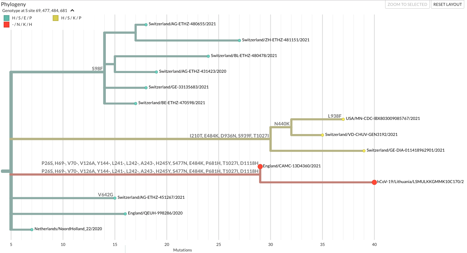
<p>The Sunday on April 11, 2021 started more or less typically - <a href="https://twitter.com/Ingridole">Ingrida Olendraitė</a> posted assembled SARS-CoV-2 genomes and their lineage breakdowns to the Slack channel we’re using with Vilnius University Hospital Santaros Klinikos. “A boring run in terms of lineages - mostly B.1.1.7 and some B.1.177.60” she said. But that changed quickly, as Ingrida pointed out that a pair of genomes in the batch gave long branch warnings in <a href="https://clades.nextstrain.org/">nextclade</a>. These two genomes - S21D420 and S21D421 - were classified by pangolin as B.1.177.57 but also had the (misleadingly sometimes called immune-evasive) S:E484K mutation. We knew S:E484K is picked up quite frequently by other lineages but the placement of these two genomes in nextclade made it clear that we weren’t dealing with anything close to B.1.177. Our mystery genomes were directly derived from a B.1-like genotype and them sitting on a long branch meant they had either been circulating somewhere undetected for a while or experienced similar selective pressures to B.1.1.7/Alpha.</p>

<p><img src="http://evogytis.github.io/files/B1620_nextclade.png" alt="Scary" /></p>

<p>The incorrect pangolin classification of these two mystery genomes as B.1.177.57 when they clearly weren’t anywhere near B.1.177 meant it would be hard to find their relatives on GISAID and the worst thing about them were the actual mutations on the long branch they sat on. It was a smörgåsbord of mutations found in classic variants of concern of the day (Alpha, Beta, and Gamma) - P26S, 69/70Δ, 144Δ, 241/243Δ, S477N, E484K, P681H, and D1118H to name the S changes alone. It looked like a cartoon villain. The mutations seemed so excessive my first instinct was to check for contamination, but that didn’t seem likely since we had two genomes, not a singleton, and Betas and Gammas that could be the source of contamination weren’t circulating in Lithuania widely. Screwing up so <em>consistently</em> seemed a bit of a stretch. Was it recombinant? We already knew those existed thanks to <a href="https://www.sciencedirect.com/science/article/pii/S0092867421009843">Ben Jackson and co</a>, but in this case we were missing a number of mutations that a B.1.1.7-derived recombinant should’ve had. So it probably wasn’t a recombinant either.</p>

<p><img src="http://evogytis.github.io/files/B1620_mutations.png" alt="Not recombinant" /></p>

<p>If we weren’t convinced by the two genomes we had at hand, we soon discovered that searching for the combination of 69/70Δ, S477N, and E484K mutations on GISAID lead to a very small (at the time) list of genomes that happened to carry the rest of the mutations too. Worse yet, that’s how we found out that another sequencing institution in Lithuania had seen this lineage a week earlier but took the pangolin B.1.177.57 label at face value and missed the S:E484K mutation. We informed government institutions to step up their game in the affected area (Anykščiai municipality) while we turned our attention to where this mystery lineage may have come from.</p>

<p>The other 30-odd genomes on GISAID with 69/70Δ, S477N, and E484K reported mid-April were from a pretty random collection of European countries: France, Belgium, Switzerland, England, and Germany, all of them collected no earlier than March 2021. An unusual lineage suddenly appearing across much of Europe was another red flag, kind of like early B.1.1.7/Alpha spread in Kent vibes. Often genomes of this lineage from the same country weren’t even closely related to each other so given the sudden appearance of these genomes across numerous European countries and that we couldn’t identify any genomes close enough to break up the super long branch leading up to these sequences led to our initial hypothesis that we were seeing something that was not endemic to Europe. Checking the data again we got our first confirmation that we were on the right track - the earliest case on GISAID was marked as a traveler returning to France from Cameroon. As luck would have it I knew the perfect group who could analyse traveler sequences in BEAST and I could certainly use more help.</p>

<p><img src="http://evogytis.github.io/files/B1620_earlyvis.png" alt="Signs of trouble" /></p>

<h2 id="unhinged-april">Unhinged April</h2>

<p>Guy Baele, Sam Hong and Barney Potter were a blessing for this project. Guy initially helped emailing folks who submitted genomes with 69/70Δ, S477N, and E484K to GISAID which by the time we were writing up had yielded a total of eight travel cases arriving from Cameroon. Sam Hong was crafting the BEAST XMLs we’d eventually use and sorted out background sequence data while Barney Potter ran analyses to look for sequences that could represent “missing links” in the evolution of our mystery lineage that could break up the long branch these genomes were sitting on. Simultaneous with these efforts we also submitted a pango lineage proposal, because listing the mutations this lineage had in every email to every new correspondent was getting tedious. To my surprise and perhaps with a lot of luck we got a pango lineage name the very next day and internally we no longer had to refer to the lineage as <a href="https://en.wikipedia.org/wiki/Puntukas">Puntukas</a> or <a href="https://en.wikipedia.org/wiki/The_Forest_of_Anyk%C5%A1%C4%8Diai">Anykščių šilelis</a> in Lithuania.</p>

<p>What followed was a 23-day writing spree that resulted in the final paper. We settled on the general outline of the study fairly quickly since there’s not much room to reinvent the wheel in a study describing a new lineage. You begin by listing the mutations it has, show some trees, describe its range, and say some things about its potential future. I struggle to remember a similar time when I knew exactly what had to be done or a time when I could work on a single project undistracted for 12 hours per day for three weeks. I would never endorse it as a healthy long-term strategy, but going to bed tired because you’re practically obsessed, able to make good progress on a project and know exactly what needs doing tomorrow is kinda nice. But only in moderation, especially because on top of actual work I was thrust into deeply unpleasant PR territory that no one else could handle.</p>

<p>At one point Lithuanian media caught wind that we had found an <a href="https://www.lrt.lt/en/news-in-english/19/1391882/unidentified-coronavirus-strain-found-in-eastern-lithuania">“unidentified” coronavirus strain</a> that I simply didn’t have time nor patience to explain to every media outlet in the country. So on I went, juggling press releases and analyses, coordinating data, and inviting co-authors while trying to ignore all the cringily awful headlines reporting on our work that verged on <a href="https://www.nature.com/articles/d41586-020-00180-8">snakerona</a> (raise your hand if you remember that story) and <a href="https://www.nature.com/articles/nature.2014.15777">Ebola mutating OMG!!1!</a>. Everyone wanted juicy scoops to write clickbait-y headlines with but no one bothered reading up on the subject matter. At one point a journalist confidently told me that “mutation” and “strain” are used as synonyms in the news and didn’t seem to know why they wanted to interview me specifically, just that there were rumours of something called “sequencing”. I wish more journalists everywhere treated their profession as a calling to knowledgably report information to society rather than just a means to collect a paycheck based on the headline clicks they get.</p>

<h2 id="visualisations">Visualisations</h2>

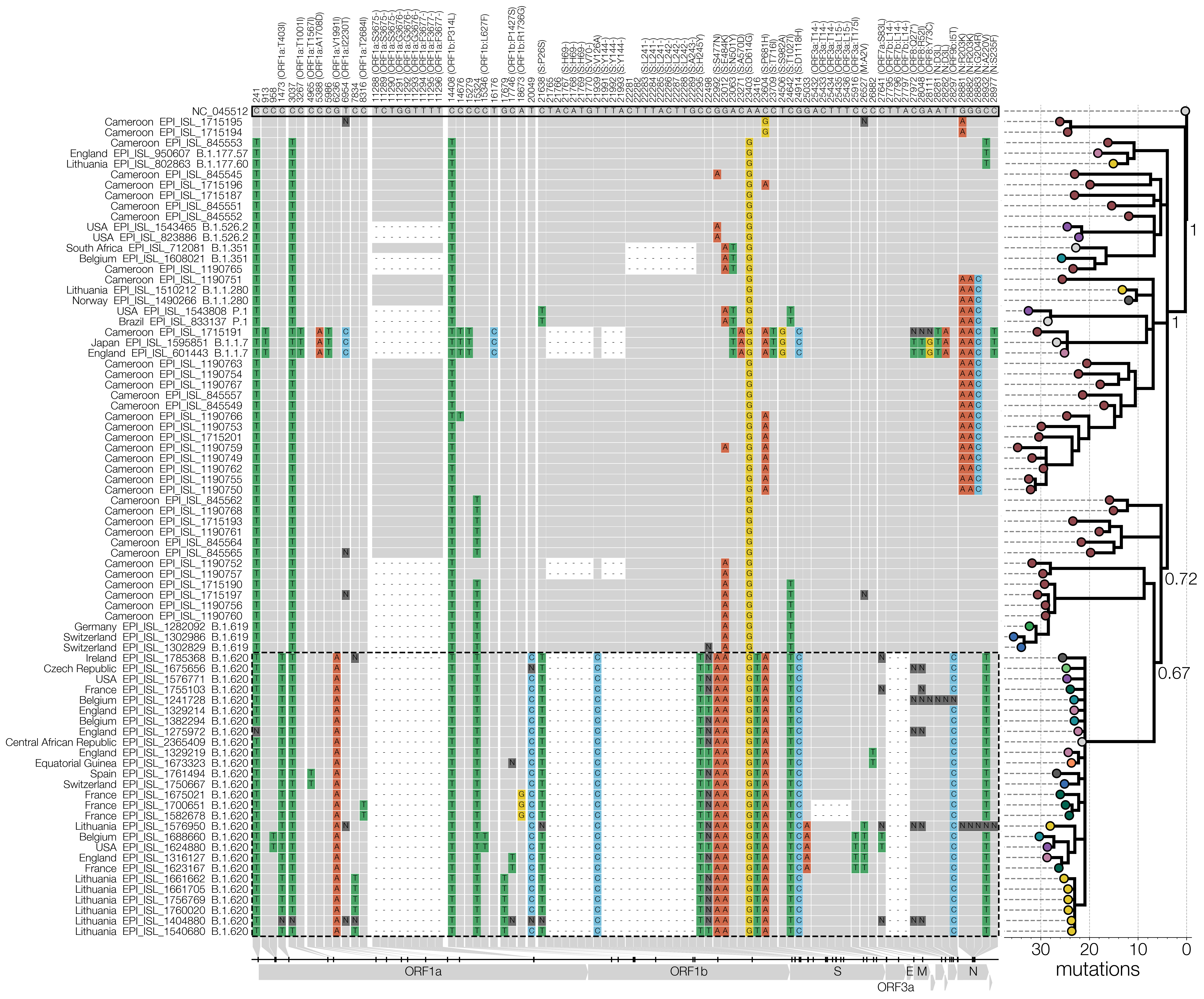
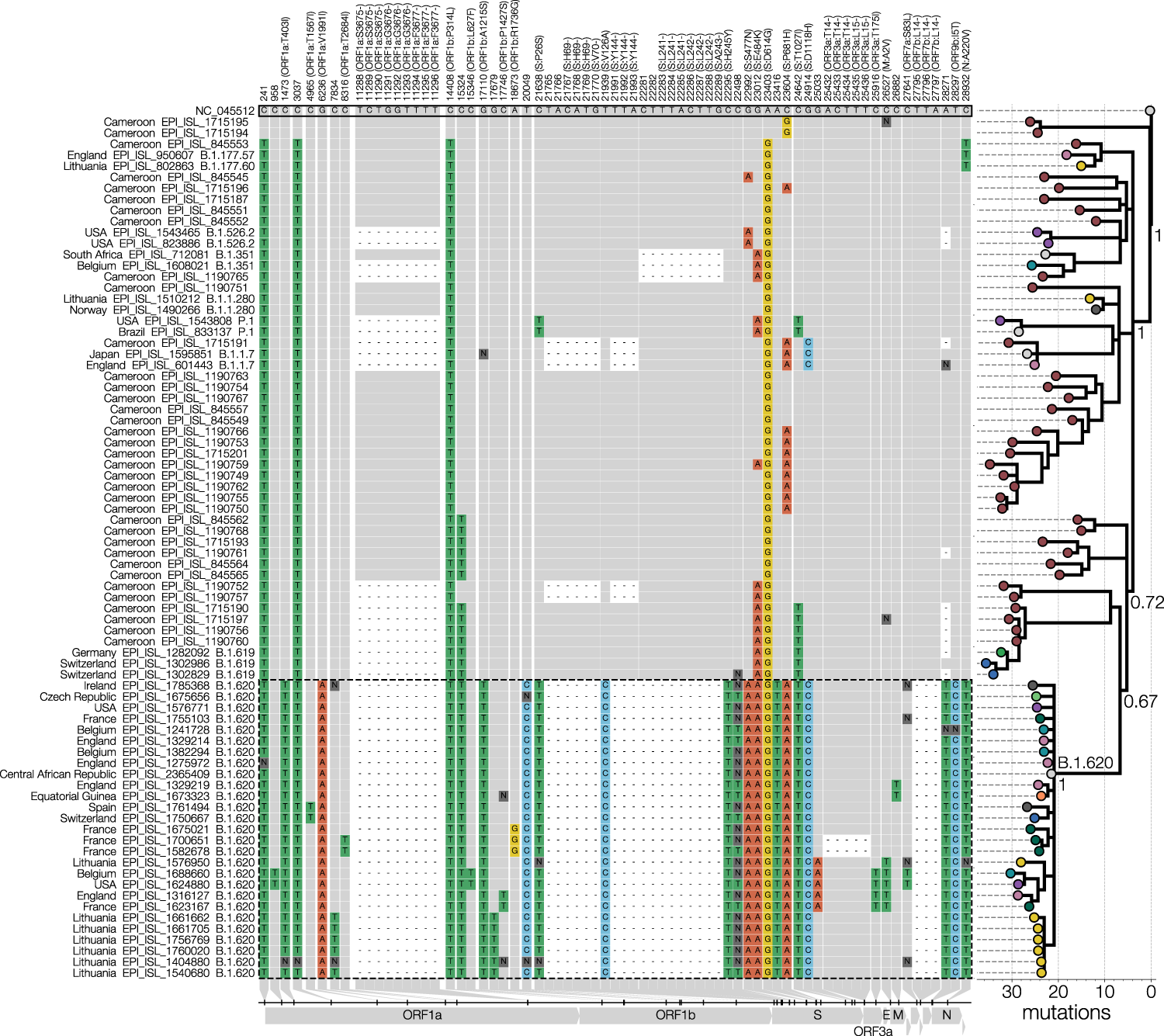
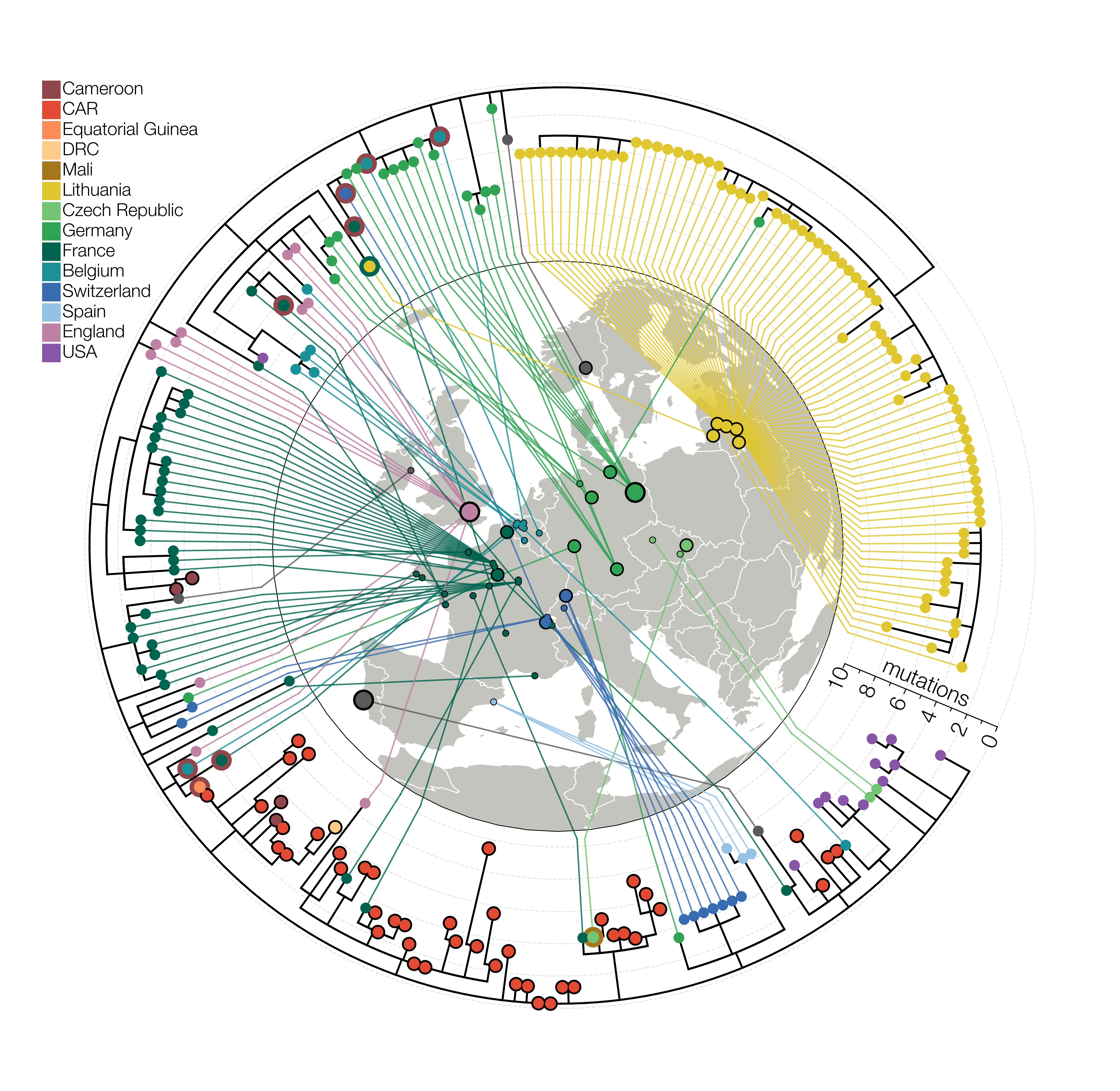
<p>Even though the paper itself was quite formulaic it did require the development of new code for visualisations that I wanted to do. Figures 1 and 2 are the only ones worth discussing here since they required the most work. Anyone who’s been following SARS-CoV-2 closely will recognise our Figure 1 as a blatant clone of <a href="https://twitter.com/AineToole">Áine O’Toole’s</a> <a href="https://github.com/aineniamh/snipit">snipit</a> visualisation with my sole contribution being the addition of a tree. I initially saw snipit in the first(?) report on <a href="https://virological.org/t/recombinant-sars-cov-2-genomes-involving-lineage-b-1-1-7-in-the-uk/658">genuine SARS-CoV-2 recombinants</a> and while I’ve done <a href="https://elifesciences.org/articles/31257#fig4s2">condensed SNP alignments previously</a> I didn’t appreciate that they could make for very informative and aesthetic figures.</p>

<p><img src="https://media.springernature.com/full/springer-static/image/art%3A10.1038%2Fs41467-021-26055-8/MediaObjects/41467_2021_26055_Fig1_HTML.png" alt="Pretty SNPs" /></p>

<p>The other thing that experts might find obvious but the novices will (hopefully) appreciate is connecting the tree to the data underlying it (the SNPs). My impression is that unless you’re working with Geneious or nowadays nextstrain/auspice, your tree-inference tool will not let you switch between the alignment and the tree or run ancestral state reconstruction, and so the tree is then somewhat divorced from its source data. I’ve seen ridiculously long branches in trees caused by misalignments and back-translated sequences that I spotted in alignments on time but I wonder how many beginner phylogeneticists not using tools that allow one to check the alignment easily would just proceed with the next steps that follow without looking back.</p>

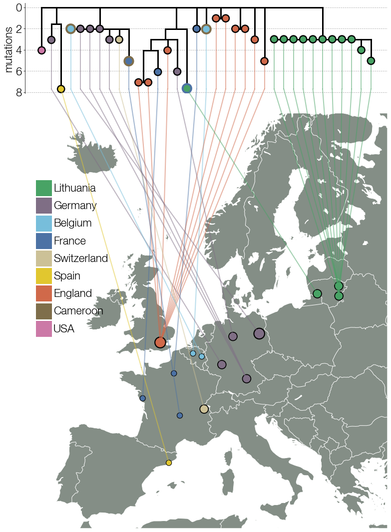
<p>Figure 2 (from earlier) was very much a clone of <a href="https://twitter.com/nidiatrovao">Nídia Trovão’s</a> figure <a href="https://academic.oup.com/view-large/figure/81461053/vev016f2p.jpeg">literally connecting trees to geography</a> which I wouldn’t know where to begin with in matplotlib until they implemented <a href="https://matplotlib.org/stable/api/_as_gen/matplotlib.patches.ConnectionPatch.html">ConnectionPatch</a>, an object that can span multiple matplotlib axes objects. When we initially had 30-odd B.1.620 genomes the figure was pretty much a carbon copy of Nídia’s.</p>

<p><img src="http://evogytis.github.io/files/B1620_earlyvis.png" alt="Signs of trouble" /></p>

<p>But at some point, as the number of genomes grew I quickly realised what I must do, I just didn’t know if I had the strength to do it. I had to go circular. It’s the one thing that myself and experienced phylogeneticists advise people not to do unless it’s for logos but I felt it was justified at the time because surrounding the map with a tree pointing inwards gave us the space we needed, it looked hip, the tree wasn’t so complicated as to be uninterpretable, it was perfect. Novel, crisp, and best of all - it told a story. But then the reviewers happened. One of the requests we received during peer-review was to include more genomes in case they changed the story. For the last six months the first thing I did in the morning was to go on GISAID to check for new B.1.620 genomes. I knew nothing new that affected our story in any way had come to light but obviously you don’t say that to reviewers. A couple of months after the initial submission there were loads more B.1.620 genomes with loads more sequencing/assembly errors which made the tree topology more complicated and the tree itself more crammed. I’m not a fan of the peer-reviewed Figure 2 we ended up with so to me Figure 2 lives in its perfect submitted form.</p>

<p><img src="http://evogytis.github.io/files/B1620_latevis.png" alt="A thing of beauty" /></p>

<h2 id="much-ado-about-nothing">Much ado about nothing?</h2>

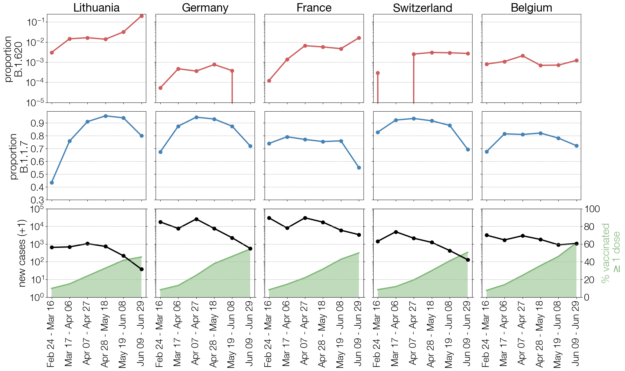
<p>We didn’t get to see if B.1.620 was all that bad thanks to B.1.617.2/Delta. There were hints from the mutations it carried and its persistence that B.1.620 probably had an advantage over B.1.1.7/Alpha in vaccinated populations that could have led to a uniquely B.1.620-dominated 2021 winter season in Lithuania. It was designated as a variant under monitoring by the ECDC together with WHO-designated variants of interest B.1.621 (WHO designation Mu) and C.37 (WHO designation Lambda) but never got its own WHO VOI designation. But in many ways the B.1.620 story wasn’t even about the lineage itself but about the failures that led to it.</p>

<p><img src="http://evogytis.github.io/files/B1620_fate.png" alt="Credible threat" /></p>

<p>Locally, I believe we spotted B.1.620 comparatively early and the call to action by some in the government was met with lukewarm efforts within institutions responsible for enacting the response. I don’t know if it was because the people responsible weren’t being paid enough to care or if the Soviet spirit of doing the bare minimum to fly under the radar was still alive and well within the institution but by the end of B.1.620’s rampage we could point to nearly 200 B.1.620 cases spread across all of Lithuania confirmed by sequencing and over 400 strongly suspected cases based on genotyping as evidence of a botched response, since all of our B.1.620 cases descended from a small outbreak in a single municipality. I wouldn’t be surprised if the responsible institutions simply didn’t understand that their failure to act on time would be clear as day in sequence data. I’m also somewhat fascinated about another independent introduction of B.1.620 into Lithuania (yes, we somehow had the sheer unluck of having two introductions) which turned out to be a traveler who as far as we could tell from sequence data did not infect anyone upon their return. By some twist of fate not only did we have an outbreak of an unusual lineage in Lithuania but we also got the perfect example of how the decisions of single individuals can have a disproportionate impact on those around us in an infectious disease setting. One person decided to self-isolate responsibly and another probably didn’t and inadvertantly led to the deaths of a number of their compatriots.</p>

<p>On a more global scale even though B.1.620 is likely to be extinct, the wider lesson it teaches doesn’t need for B.1.620 to still be circulating. We often talk about global inequalities that rob poorer countries of opportunities but when we argue that it’s a problem we frequently have to rely on evidence from absence. Absence of comparable numbers of scientists, papers, institutions, <em>etc</em> coming from poorer countries. I think B.1.620 was an interesting twist on this argument. The lack of vaccines in central Africa probably allowed B.1.620 to evolve in the first place while the lack of sequencing there robbed richer countries of an early warning that B.1.620 even existed until it was knocking on our door. Everyone ended up losing and it didn’t matter that the Baltic states and central Africa are about as random as any two locations in the world can get. The <em>de facto</em> world we find ourselves living in is considerably smaller than it used to be, it has been for a while, and it gets smaller every year. We can continue pretending that problems elsewhere aren’t ours but reality will call this bluff every time, to our disadvantage.</p>

<h2 id="the-other-dream-teams">The other dream team(s)</h2>

<p>Although Guy, Sam and Barney did most of the heavy lifting for our B.1.620 study I would also like to acknowledge the folks whose work enabled us to do so in the first place. I have to thank <a href="https://twitter.com/ingridole?lang=en">Ingrida Olendraitė</a> for getting me involved in Lithuania’s pandemic response at the end of 2020. Ingrida had been an irreplaceable left hand (#teamLeftie) in everything to do with Lithuania’s SARS-CoV-2 sequencing project while still writing up her thesis. It’s been an honour and a pleasure to work with such a promising young scientist and I’m already looking for ways to continue collaborating. When the government was finally ready to fund the sequencing project, writing the actual genomic surveillance project proposal could not have happened without the help of <a href="https://www.researchgate.net/profile/Rimvydas-Norvilas">Rimvydas Norvilas</a>, <a href="https://lt.linkedin.com/in/dovil%C4%97-juozapait%C4%97-095aa9216">Dovilė Juozapaitė</a>, and <a href="https://lt.linkedin.com/in/daniel-naumovas-3a9708167">Daniel Naumovas</a>. While Ingrida and I worked on the “why do this” and “what needs to happen” aspects of the project they worked out all of the technical details. When the sequence data were finally rolling in it quickly became apparent that government institutions needed a person who could clean the metadata. Luckily for us <a href="https://twitter.com/MGabrielaite">Miglė Gabrielaitė</a> stepped up to the challenge and volunteered her time despite being in the final stages of her PhD and expecting. <a href="https://lt.linkedin.com/in/aistissimaitis">Aistis Šimaitis</a> from the government’s chancellery and <a href="https://lt.linkedin.com/in/jonas-ba%C4%8Delis-a848ba20a">Jonas Bačelis</a> from the government’s statistics department were crucial for coordinating the data infrastructure required to pull off a project with this amount of throughput and numerous other scientists working at Vilnius University Life Sciences Center, Lithuanian University of Health Sciences, Vilnius University Hospital Santaros Klinikos, and Lithuanian University of Health Sciences Hospital Kauno Klinikos also contributed the key ingredient to our study - Lithuanian SARS-CoV-2 genomes. Since this study came out I’ve moved back to Lithuania and I couldn’t have asked for a better way for the Lithuanian science community to get to know me and <em>vice versa</em>.</p>

<p>Though getting sequencing up and running in Lithuania was a challenge in many ways, some of the hurdles that inconvencienced us somewhat (and probably would’ve been easy to solve in richer countries) obviously had to present substantial challenges for groups sequencing in Africa. To date the closest relatives of lineage B.1.620 - its sibling lineage B.1.619 and intermediate precursor-looking lineages were found in Cameroon and were sequenced, as far as I can tell, because <a href="https://scholar.google.com/citations?hl=en&amp;user=5g4P-18AAAAJ">Ahidjo Ayouba</a> took the initiative to do so. It highlights yet again that sequencing regularly, regardless of how boring the current state of the epidemic looks, can contextualise future sequences in unforeseen and informative ways. Similarly, as we were writing up the B.1.620 story, numerous groups around Africa were able to get their samples sequenced and submitted to GISAID, often with the help of <a href="https://inrb.net/">INRB</a>, who have time and again stepped up to do necessary sequencing in DRC (and abroad this time). I’m very glad we were able to add the names of researchers who sequenced B.1.620 in Africa to the paper to acknowledge their efforts.</p>

<h2 id="a-short-note-on-impostor-syndrome">A short note on impostor syndrome</h2>

<p>Most scientists encounter impostor syndrome in one way or another at some point in their careers and I’m no exception. A superior can reassure us that we’re on the right track and discussing our work with colleagues helps us approach problems from a wider set of angles and get more minds working on the problem. Since leaving Seattle in the summer of 2018 I haven’t had the luxury of either but I managed to cope okay because I was working on RNA virus discovery projects proceeding at their own pace. SARS-CoV-2 work, on the other hand, required a degree of urgency and precision. My happiness at making predictions based on limited data might seem childish to the experienced phylogeneticist because in retrospect the initial observations <em>were</em> quite obvious, but trusting my own abilities to make inferences in the absence of superiors and colleagues telling me “yes, that makes sense” took a lot of effort. Though I’m nowhere near “cured” of my impostor syndrome at least I got some vaguely objective evidence for why I’m not completely useless.</p>]]></content><author><name>Gytis Dudas</name><email>gytis.dudas@gmc.vu.lt</email></author><category term="genomic epidemiology" /><category term="SARS-CoV-2" /><summary type="html"><![CDATA[You might’ve heard the unofficial motto of the SARS-CoV-2 pandemic - no one is safe until everyone is - floating around. Folks working in infectious disease understand it viscerally but I’m sure many outside the field still think it’s just some hippy slogan. So in this blog post I will tell you the story of SARS-CoV-2 lineage B.1.620 that landed on my lap thanks to a bit of (un)luck and a whole lot of globalisation. I figured that what transpired with lineage B.1.620 was somewhat unique and serves as a blunt statement about the planet we find ourselves on and how our failure to acknowledge that leads to a continuing cycle of avoidable mistakes. So let’s start at the beginning.]]></summary></entry><entry><title type="html">Reassortment networks and why I think they’re cool</title><link href="https://evogytis.github.io/posts/2020/10/reassortment/" rel="alternate" type="text/html" title="Reassortment networks and why I think they’re cool" /><published>2020-10-05T00:00:00+03:00</published><updated>2020-10-05T00:00:00+03:00</updated><id>https://evogytis.github.io/posts/2020/10/reassortment</id><content type="html" xml:base="https://evogytis.github.io/posts/2020/10/reassortment/"><![CDATA[<h3 id="why-youre-reading-this">Why you’re reading this</h3>

<p>This blog post will be a bit unusual. Normally I’d like my blog posts to present the “behind the scenes” context for papers that explain the logic of certain decisions whilst also explaining papers casually. This blog post will be very different as I did not play a key role in the paper I’m about to discuss (I’m a co-author though). You may have noticed that on my website I split the papers I’ve been on into “publications” and “contributions”. What I call publications are papers that wouldn’t have materialised or wouldn’t have materialised in their shape had I not been on board. The papers I refer to as contributions are for cases where I wrote some code, made a figure or ran some analysis but wouldn’t feel comfortable calling my own. While <a href="https://www.pnas.org/content/117/29/17104">Nicola Müller’s new paper on reassortment networks</a> is distinctly a contribution for me I think it has potential to impact the field in profound ways and thus should be popularised more widely.</p>

<h2 id="what-is-reassortment">What is reassortment?</h2>

<p>Reassortment and I go way back. If the West African Ebola virus epidemic hadn’t gotten me involved in a bewildering array of papers my first first-author piece of published scientific research would’ve been on reassortment in human influenza B viruses (a topic that deserves its own blog post eventually). Reassortment is a special case of recombination that occurs in viruses whose genomes are split across physically unlinked RNA molecules referred to as segments. If two or more genetically distinct viruses coinfect the same cell the progeny virions coming out of the cell can contain a mixture of segments from different parents. Influenza viruses are perhaps the most widely known examples of segmented viruses, but there are plenty of other examples too (<em>e.g.</em> Partitis, Rotas, Bunyas, <em>etc</em>). In RNA viruses that are positive singled-stranded or double-stranded recombination can occur on top of reassortment, but for the most part everyone analyses segments as independently evolving fragments, so basically like recombination with known breakpoints.</p>

<p>Reassortment is overwhelmingly important for generating pandemic influenza viruses. Most of 20th century pandemics were caused by seasonal human influenza A viruses swapping a couple of their segments for avian influenza A virus counterparts. The segment coding for the surface protein haemagglutinin (HA) would always be swapped out in pandemic viruses, suddenly making them completely new in the eyes of everyone’s immune system. The way we know these things is by building trees of every segment and seeing where each sample falls across the 8 (for influenza A and B) segment phylogenies and reconstructing in our mind’s eye what tree operations could turn one segment’s tree into another. It’s a modestly complicated exercise that needs to happen after every influenza pandemic and it’s quite entertaining. It also leads to cool graphics.</p>

<p><img src="https://media.springernature.com/full/springer-static/image/art%3A10.1038%2Fnature08182/MediaObjects/41586_2009_Article_BFnature08182_Fig1_HTML.jpg?as=webp" alt="Choo choo" /></p>

<p>Once we’re done figuring out how a pandemic originated you probably want to shift focus to phylodynamics of the new virus on the human side. Since the virus appears new to population level immunity the virus explodes in numbers, making the viral population quite homogenous during its first sweep. Since there’s not much diversity to speak of and the virus hasn’t had much time to circulate around most people won’t have co-infections, let alone co-infections with genetically distinct strains, few would complain if you ditched the multi-tree approach to sequence analysis and treated the entire genome as a single clonal block. A couple of years later when there’s enough accumulated diversity across segments and the occasional reassortment is when you should go back to using multiple trees to look at our imaginary pandemic influenza virus. In this blog post I will argue that not only is this analysis approach no longer needed but that it is good we don’t.</p>

<h2 id="overparameterising-evolution">Overparameterising evolution</h2>

<p>In my <a href="https://academic.oup.com/ve/article/2/1/vev023/1753363">MERS-CoV recombination paper</a> I made the observation that despite abundant and overwhelming evidence of recombination in MERS-CoV genomes analysing MERS-CoV sequences as either a single clonally evolving block or two blocks split across a statistically significant breakpoint evolving independently on two trees, the former clonal model fit the data much better according to marginal likelihood estimates. The rationalisation then (and now) is that recombination in MERS-CoV is just a light peppering of homoplasies across numerous branches, so adding the extra tree (that’s at least another N*(N-1) parameters to infer) overparameterises the “clonal lite” model of MERS-CoV evolution we postulated and thus a single tree is sufficient to explain the data.</p>

<p>For detectable reassortment to occur in influenza viruses there must be co-infection of a single host not only with genetically distinct viral genomes but co-infection with reassortment-compatible viral lineages. Influenza A and B viruses are far too diverged to reassort naturally and even <a href="https://www.sciencedirect.com/science/article/pii/S0042682202915138">human-origin inter-subtype influenza A reassortants don’t fare so well</a>. This is a roundabout way of saying that in human influenza co-infection is not the norm - an influenza virus will usually depart a human host with whatever segments it arrived with, perhaps sprinkled with a few new mutations. Each time we add a new segment tree to the analysis we’re introducing at least N*(N-1) parameters in an attempt to accommodate a small number of reticulate branches.</p>

<p>You might remember <a href="https://evogytis.github.io/posts/2020/01/horizon/">my previous blogpost</a> or <a href="https://bmcevolbiol.biomedcentral.com/articles/10.1186/s12862-019-1567-0">paper</a> where I talked about the rate at which mutations are observed in alignments of different lengths and evolving under different rates. There we chose to quantify the ability of mutations to resolve time by estimating the mean waiting time to a mutation as a function of evolutionary rate R across an alignment with L sites, which ends up being 1/RL. The shorter the mean waiting time to a mutation the more informative the dataset about the passage of time, like stopwatches are more informative than wristwatches because stopwatches have a millisecond hand that wristwatches don’t. It’s nearly guaranteed that best resolution with sequence data is achieved when you analyse full genomes and even then most RNA viruses accumulate mutations on the order of weeks. To maintain the same resolution (mean waiting time to mutation) a shorter alignment needs to evolve at a rate 1/f faster than the full genome where f is the fraction of the genome. You can see the problem already.</p>

<p>If you take the <a href="https://royalsocietypublishing.org/doi/10.1098/rsbl.2013.0331">genome-wide evolutionary rate</a> and genome length of the 2009 H1N1 pandemic influenza virus (3.4*10^-3 subs/s/y and 13kb, respectively) you expect the mean waiting time for a mutation to be around 8 days. You can think of this term as the lower bound on the error of a well-calibrated molecular clock model. Unless you’re using some next generation phylogenetics you cannot escape the uncertainty of around 8 days when dealing with a dataset of this length evolving at this evolutionary rate. When you reduce the alignment length by analysing sequence data one segment at a time you’re losing statistical power. Your 8 day uncertainty that you could do nothing about turns to 2 months of uncertainty. The confidence intervals around the timings of your segment tree nodes would increase around 8-fold from the genome-wide tree.</p>

<p>Finally there’s another overlooked problem that only arises in certain analysis setups. If you’re running a molecular clock tree you’re also picking a tree prior. If you choose to give each of your segments an independent tree prior you run into the problem of not having enough sites per segment to be very informative. Linking the tree priors into a single model seems like the right thing to do, but as Nicola found out it’s actually terrible. While introducing extra trees to explain largely clonal data might be overparameterising, treating the then poorly-informed tree nodes as independent data in a coalescent framework ends up double counting the data. If we believe that influenza virus evolution is mostly clonal then coalescences mostly represent whole-genome transmission events. Clusters of coalescences across all of our “independent” loci can only be interpreted as extremely low effective population size by the coalescent. Empirical data agree.</p>

<p><img src="https://www.pnas.org/content/pnas/117/29/17104/F2.large.jpg" alt="Uh oh" /></p>

<h2 id="reassortment-networks">Reassortment networks</h2>

<p>Specifying a new statistical model is relatively easy compared to writing code to efficiently explore new parameter spaces with MCMC. Clonal tree operations alone move the tree through some pretty complicated spaces so you can imagine how difficult it must be to write something that efficiently traverses space that has even more dimensions. The data structure that gets sampled during MCMC is a tree that contains tip-like edges that carry the genetic material of some segments to another branch. If you wanted to recover the descent of any given segment you would traverse back from a tip of interest back towards the root unless the branch being traversed contains a reassortment contribution that carried the segment in question, in which case you’d switch your traceback towards the root from where that reassortment edge descended. When visualised reassortment networks are dense with information but ultimately not the easiest to interpret, especially if you want segment-level information.</p>

<h2 id="visualisation-challenges">Visualisation challenges</h2>

<p>Visualising reassortment networks as trees with edges of a different kind is relatively easy, but I struggled at first to think of <em>useful</em> things to highlight. Highlighting clonal parts of the tree (<em>i.e.</em> evolution between reassortment events) seemed like a good idea and the first thing I tried was making an <a href="https://www.ncbi.nlm.nih.gov/pmc/articles/PMC5712493/figure/F4/">exploded tree</a> equivalent where each clonal section of the tree would be offset along the y-axis. Since you’re not seeing it here I didn’t think it worked very well. Networks are messy to begin with and moving away from a tree-like layout with reassortment edges criss-crossing just seemed to strain the eye too much. What I did instead is colouring branches a new colour after a reassortment event using a non-intrusive cycle of sequential colours (like <a href="https://doi.org/10.6084/m9.figshare.11466801.v1">this</a> but less vivid) which I thought did the job relatively well:</p>

<p><img src="https://www.pnas.org/content/pnas/117/29/17104/F3.large.jpg" alt="It's alright" /></p>

<p>The next challenge was reassortment edges. In Nicola’s paper I chose to display these as lines that represent each reassorting segment as a line of a particular colour:</p>

<p>I think that works fine, though I’ve also experimented with highlighting segments with a row of binary boxes (bottom):</p>

<p><img src="https://www.biorxiv.org/content/biorxiv/early/2020/02/12/2020.02.10.942854/F7.large.jpg" alt="A new era" /></p>

<p>And finally one can continue sticking with multiple trees, but highlighting the clonal path of each segment:</p>

<p><img src="http://evogytis.github.io/files/fluB_reassortment_network_untangled.png" alt="Somewhat clearer" /></p>

<p>Obviously, I’m still trying to find better ways of visualising these and I’m very open to suggestions.</p>

<h2 id="the-potential">The potential</h2>

<p>So far I’ve been talking about how reassortment networks are better at utilising information and how annoying it is to plot them in a satisfactory way. I now invite you to imagine the possibilities of what is possible.</p>

<h3 id="more-power">More power</h3>

<p>In order for reassortment to occur two viral genomes must find themselves in the same cell. If two viral genomes are in the same cell you can be sure they’re in the same geographic location too, so if you were able to run something like your typical discrete trait analysis on top of a reassortment network you’d be leveraging the same levels of information that we gained access to in molecular clock analyses. We’re talking more power to infer timings and more power to infer state transition rates, so what’s not to love?</p>

<h3 id="reassortment-distance">Reassortment distance</h3>

<p>In my 2014 <a href="https://academic.oup.com/mbe/article/32/1/162/2925578">influenza B reassortment paper</a> I used a metric called 𝛿TMRCA. It was the difference in most recent common ancestor dates for the same pair of tips in two different segment trees. The idea is that if the two numbers are really different the more recent TMRCA will correspond to a reassortment (because one of the lineage’s evolutionary history was overwritten by an incoming lineage) and the older TMRCA is a genuine common ancestor (though it could be another reassortment event too). That distance is meant to represent the amount of independent evolution that has occurred between two segments since they were part of the same genome until they encountered each other again in a reassortant genome. Alternatively you can think of it as your reassortment signal - genomes reassorting after diverging for a month are likely to be identical (and thus reassortment undetectable), but segments reassorting between genomic backgrounds that have been diverging for decades would be very easy to spot. This is in fact what Nicola and co showed in their Figure 1C:</p>

<p><img src="https://www.pnas.org/content/pnas/117/29/17104/F1.large.jpg" alt="Funky and cool" /></p>

<p>Depending on the limitations of the system you could look at the rate at which different parts of the same viral genome diverge epistatically, <em>i.e.</em> the rise of <a href="https://en.wikipedia.org/wiki/Bateson%E2%80%93Dobzhansky%E2%80%93Muller_model">Dobzhansky-Muller incompatibility</a>. I described an example of this type of incompatibility in my influenza B reassortment paper (<a href="https://rdcu.be/b5AtI">later confirmed in cell culture</a>) and Villa &amp; Lässig <a href="https://doi.org/10.1371/journal.ppat.1006685">described this in much finer detail for influenza A viruses</a>.</p>

<h3 id="co-reassortment">Co-reassortment</h3>

<p>Obviously the other thing that you can look into using Nicola and co’s method is co-reassorting segments. We convinced ourselves that co-reassorting PB1-PB2-HA segments in influenza B were the result of post-reassortment selection on hybrid PB1-PB2-HA segment constellations, but another possibility is that co-reassortments occurs via some peculiarity of the segment packaging mechanism. Barring intensive analyses of gigantic sequence datasets or exhaustive cell culture experiments there’s no easy way of seeing if segments are co-reassorting. For something with 8 segments like influenza A and B there are 254 different kinds of reassortants (2^8-2, where you pick whether a given segment was reassorted or not minus where all segments are derived entirely from one or the other parent) that can be produced from a co-infection. To establish statistically significant differences in observation rates between particular segment combinations you clearly need very high numbers of reassortments. While this doesn’t apply to specific hypotheses (<em>e.g.</em> particular labeled lineages do not reassort across a defined number of potential reassortment opportunities) it makes exploratory analyses unfeasible. As such, despite my optimism about reassortment networks in general I believe this one is an inherent limitation of the data that no method can solve easily.</p>

<h3 id="unforeseen-cases">Unforeseen cases</h3>

<p>I can’t help but approach reassortment and what I’d like to learn about the process with the personal biases that brought me to the topic in the first place. So if I have missed a potential avenue of research do tell me so I can update this section of the blog post!</p>

<h2 id="final-thoughts">Final thoughts</h2>

<p>We may be in the middle of a coronavirus pandemic in the year 2020 but let’s not forget the other F word that comes to mind when we talk about pandemics - flu. <strong>When</strong> the next influenza pandemic hits I’m hoping that Nicola’s reassortment network model will have been picked up, improved upon and deployed widely, simply because it’s the only method that maximises sequence data use and reduces the amount of data post-processing in segmented datasets. To summarise, if you have all segments of a measurably evolving virus and you want the best possible segment trees under the constant population size coalescent tree prior you can’t do any better right now than reassortment networks™.</p>]]></content><author><name>Gytis Dudas</name><email>gytis.dudas@gmc.vu.lt</email></author><category term="virus evolution" /><category term="influenza virus" /><summary type="html"><![CDATA[Why you’re reading this]]></summary></entry><entry><title type="html">Why are sundials not used on GPS satellites?</title><link href="https://evogytis.github.io/posts/2020/01/horizon/" rel="alternate" type="text/html" title="Why are sundials not used on GPS satellites?" /><published>2020-01-23T00:00:00+02:00</published><updated>2020-01-23T00:00:00+02:00</updated><id>https://evogytis.github.io/posts/2020/01/horizon</id><content type="html" xml:base="https://evogytis.github.io/posts/2020/01/horizon/"><![CDATA[<h2 id="a-short-introduction">A short introduction</h2>

<p>This blog post is about a recent paper that just came out in <a href="https://bmcevolbiol.biomedcentral.com/articles/10.1186/s12862-019-1567-0">BMC Evolutionary Biology</a> which happens to be the last bit of work left from my time with <a href="http://bedford.io">Trevor Bedford’s group</a> in Seattle.
The paper came about as a bit of an emergency when I learned that I wouldn’t be able to come back to US if I decided to leave after January 2018 due to my visa expiring and my desire to replicate the success of <a href="https://academic.oup.com/mbe/article/23/1/7/1193608">a highly cited paper that was written in 24 hours</a>.
An idea about a paper like this had been floating around my head for a while ever since Pardis Sabeti and a few others asked where a figure I had used in a talk was published (it wasn’t) and given the interest it sounded like such a paper would make for an excellent citation cow.</p>

<p>The study focuses on something that’s been discussed by many other groups before (<em>e.g.</em> <a href="https://journals.plos.org/plospathogens/article?id=10.1371/journal.ppat.1006885">Thibaut Jombart et al</a> and <a href="https://www.nature.com/articles/s41564-018-0296-2">Nathan Grubaugh et al</a>) and <em>should</em> be intuitive but, as it turns out, is worth repeating often.
What sequences can tell you about their history is highly dependent on how fast they evolve and how much of the sequence you look at, but let’s delve a bit deeper.</p>

<h3 id="the-basic-principles-of-phylodynamics">The basic principles of phylodynamics</h3>

<p>Phylodynamics is probably best described as a sub-sub-field of phylogenetics that focuses on analysing genetic sequences of microbial organisms by reconstructing their history (the phylogenetic tree) and trying to say something about the processes that generated/shaped the phylogeny.
When done right it can yield exquisite detail about the organisms being studied, often at a fraction of the cost that alternative methods (<em>e.g.</em> contact tracing or lab testing) would incur.
Many bigger food-borne disease outbreaks these days, for example, are likely to be tackled by sequencing and comparing infectious agents from human cases and food items from specific farms, rather than waiting until there’s conclusive evidence linking human cases to contaminated food from a specific farm or testing all possible farms simultaneously.</p>

<p>At the core of these phylodynamic/genetic epidemiological approaches is the fact that microbes tend to have short generation times (<em>i.e.</em> they replicate often) which leads to more replication errors (mutations) happening in the genome of the organism.
One can consider every mutation as a unique marker of a lineage which gets inherited by all of its descendants.
Genomes descended from a modified/mutated genome can in turn be marked with additional mutations (that their sibling or parental lineages do not possess) and as long as mutations are not overwritten or reverted back they will record the history of descent of all lineages.
The job for phylogenetic methods is to reverse-engineer the process of modification and inheritance by establishing which mutations seen in sequences are likely to be shared because they were inherited from a common ancestor and which happened to occur at the same genomic site independently (rare in the absence of strong selection, difficult in the presence of recombination).
But how much the phylogenetic tree can tell you about the organism whose history you’re interested in depends on the timescale of the process in question and the rate at which mutations are generated and observed in the organism’s population.</p>

<h3 id="temporal-resolution-and-the-genomic-horizon">Temporal resolution and the genomic horizon</h3>

<p>The steady accumulation of predominantly neutral sequence variation in organisms over time is modelled via molecular clocks.
To put it very simply these models infer the passage of time from the random ticks of the mutation clock (subject to sequence sampling relative to diversity) or, to rephrase, molecular clocks identify plausible timeframes long enough for a mutation to have occurred in.
Because things like RNA virus populations accumulate mutations rapidly it is usually sufficient to sample tens of genomes collected a couple of years apart to get a good estimate of the rate at which mutations were generated and spread through the population to a sufficient frequency to be observed.
Molecular clocks can be very precise if they are given large numbers of mutations and the two ways of getting more mutations in your sample is pretty simple - increase the rate at which mutations are observed (possible because selection is usually not uniform across sites) or increase the number of sites you are observing.</p>

<p>Back in the day the limitations of sequencing technologies made it obvious which of the two strategies (more sequences versus more sites) is more feasible.
Sequencing lots of sites was too expensive and/or too laborious and therefore the regions evolving fastest (or conversely alignment regions that looked most diverse) would be sequenced with higher priority as they offered the most potential to differentiate any two given lineages.
Barcoding of pathogen sequences proliferated as a result.
Just as a reference there are at least 5000 sequences of a tiny gene called SH of mumps virus (512 nt) on GenBank and only 249 complete genomes (&gt;15,000 nt).</p>

<p>While having more data sounds like a great idea one should also be aware of any implicit trade-offs.
This entire study started because of a rather simplistic model of sequence evolution that Andrew Rambaut used in a blog post to argue that a small sequence fragment of “the closest thing to MERS-CoV” in an Egyptian bat could have been around unchanged for ~5 years, making it unlikely to be that close to MERS-CoV and therefore not quite the find it was made out to be.
As you’ll see later this simple model in addition to being a cool way of thinking about sequences also has grave implications for phylodynamic study data generation strategies and suggest that you too should be worried about short sequences appearing on NCBI in large numbers.</p>

<h3 id="a-bit-of-maths">A bit of maths</h3>

<p>Here’s how the model goes - assume that mutations are a Poisson process (discrete events occurring randomly over time).
The waiting time for a Poisson process is exponentially distributed and so the probability of a mutation not happening over time depends on the rate at which mutations occur (this is exactly the same maths used for radioactive decay).
Let’s express the probability <em>p</em> that a mutation does not happen at a site after time <em>t</em> under evolutionary rate <em>R</em> as</p>

<p><img src="https://latex.codecogs.com/gif.latex?p=e^{-Rt}" alt="No mutation" /></p>

<p>We’re more interested in the probability <em>p</em> that at least one mutation happened at the site evolving at rate <em>R</em> after time <em>t</em> because that tells us when two lineages are likely to become distinguishable, which is</p>

<p><img src="https://latex.codecogs.com/gif.latex?p=1-(e^{-Rt})" alt="At least one mutation" /></p>

<p>We assume that this process occurs independently across all sites of an alignment, which we’ll complicate a bit.
Let’s assume that you have a genome of length <em>G</em> but for financial reasons you can only afford to sequence a fraction <em>f</em> of the sites, giving you an alignment length of <em>L</em> (L=Gf).
The probability <em>p</em> of observing at least one mutation in an alignment of length <em>L</em> evolving at rate <em>R</em> after time <em>t</em> is</p>

<p><img src="https://latex.codecogs.com/gif.latex?p=1-(e^{-RLt})" alt="At least one mutation in L sites" /></p>

<p>We’ll simplify this a bit by saying that we don’t actually care about specific waiting times <em>t</em> (or any specific probability <em>p</em> that at least one mutation has occurred for that matter) and instead are interested in the mean expectation for a given rate <em>R</em> and alignment length <em>L</em>.
For a simple exponential distribution e^λ the mean expected value is 1/λ and for our purposes we can think of <em>RL</em> as λ and so the mean expected time to at least one mutation becomes 1/RL.
Much like it is far more useful to describe radioactive decay by a single parameter called half-life (the waiting time until only half of radioactive atoms are left) rather than the full probability distribution that tells you the probability of any given atom decaying after some amount of time, in our case it is much easier to think about 1/RL (two parameters) rather than the whole distribution (four parameters).</p>

<h3 id="the-genomic-horizon">The genomic horizon</h3>

<p>So for now we have a parameter 1/RL which is the mean waiting time for at least one mutation to occur in an alignment of length <em>L</em> evolving at rate <em>R</em>.
As someone doing phylodynamics you want to minimise 1/RL (you don’t want to wait a long time for mutations) as much as possible and increasing either <em>R</em> or <em>L</em> will do the trick - if you increase <em>R</em> mutations crop up more often and if you increase <em>L</em> you’re more likely to spot mutations because you’re looking at more sites.
Here’s a pretty important empirical observation that should make you worried - both <em>R</em> and <em>L</em> have upper limits.
Organisms tend to have an upper bound on evolutionary rate <em>R</em> because of deleterious mutation load while <em>L</em> is capped by genome length (<em>i.e.</em> <em>L</em> is strictly ≤<em>G</em>).
This is what I refer to as the genomic horizon of sequence data - every evolving genome will have an upper limit on how frequently on average mutations will be observed in it and thus there will be a limit to how fast information can be encoded in a phylogeny.
In the same way that one wouldn’t rely on mutations accumulating in humans generation-to-generation to assess the rate of modern transcontinental travel one wouldn’t dream of using 5 sites from a viral genome in a who-infected-whom study.</p>

<p>To get a sense of what combinations of alignment length <em>L</em> and evolutionary rate <em>R</em> do to temporal resolution here’s the figure that started this entire study (including some usual suspects):</p>

<p><img src="https://raw.githubusercontent.com/blab/genomic-horizon/master/figures/fig6_contours.png" alt="Look at them contours and despair" /></p>

<p>Almost every virus is capped at around one mutation every ~3 weeks and the few things that exceed that threshold, mainly influenza A (very high evolutionary rate and moderate numbers of sites) and MERS-CoV (a very long genome and moderate evolutionary rate), are made more difficult to analyse because both evolve non-clonally to some extent (reassortment and recombination, respectively).
In turn this means that processes occurring faster than those timeframes are impossible to encode with any fidelity in viral genomes.</p>

<h3 id="the-futility-of-partial-sequences">The futility of partial sequences</h3>

<p>The evolutionary rate parameter <em>R</em> we’ve been talking about is something that researchers get to pick from a limited range of values, but never fully control.
One way of increasing <em>R</em> is to sequence very intensely because it captures circulating deleterious variants that will get purged from the population eventually.
You can also find regions of the genome that evolve faster than average, but for a variety of population genetics reasons you’re unlikely to ever encounter a region that will fully compensate the temporal resolution that you lost by not sequencing complete genomes.
Let’s come back to our mean waiting time for at least one mutation (1/RL) and express <em>L</em> as <em>Gf</em> (genome length times fraction sequenced), which becomes 1/RGf.
Assume that we have identified a single contiguous region comprising 10% of the genome that evolves at a rate twice as fast as the genomic average which sounds sweet!
But then keep in mind that whatever’s been lost in <em>G</em> (genome length) because <em>f</em> (fraction that’s sequenced) is reduced needs to be made up for by <em>R</em> (evolutionary rate).
In order to maintain the temporal resolution that full genomes allowed the 10% (f=0.1) that we’re sequencing would need to evolve at a rate that’s 1/<em>f</em> higher than the genomic average <em>i.e.</em> 10 times faster.
Even for moderate values of <em>f</em> the speed up in <em>R</em> required to maintain the temporal resolution available with complete genomes is excessive - for 40% of the genome (f=0.4) evolutionary rate <em>R</em> needs to be 2.5 times higher (which is still unrealistic for site-wise rate heterogeneity) and by the time you’re sequencing 40% of the genome you might as well be sequencing the remaining 60%.</p>

<p>The lesson here is that more sequences do not always mean more information.
If your aim is to know how many cases of something are caused by lineage A or B then sequencing 100 000 sequences that are 100 nt long might be a perfectly valid approach, but you would definitely want to sequence 1000 sequences that are 10 000 nt long if you cared about anything more than just what organism you’re sequencing.
Even then there will be a limit, a horizon, to what genomic data can tell you about processes that occur faster than the rate at which genomes are made different by mutations.</p>

<h2 id="empirical-tests">Empirical tests</h2>

<h3 id="methods">Methods</h3>

<p>To demonstrate/test the effect of reducing alignment length on inference we decided to use a traditional machine learning type method of train-test split.
We took 1610 Ebola virus genomes (~19,000 nt long) from our <a href="https://www.nature.com/articles/nature22040">earlier study</a>, kept only those that didn’t have too many ambiguous sites and where we knew where (down to 2nd admin level) and when (year-month-day) it had been collected.
That still left us with ~900 sequences so we additionally down-sampled this to 600 genomes and picked 60 of those at random which would be our test set.
We pretended that we didn’t know when and where those 60 sequences were collected.
Then we produced a secondary dataset from the 540 training and 60 testing genome sequences by extracting just the glycoprotein (GP) gene (~2000 nt long).
Though a variety of Ebola virus genes had been used as markers in the past GP probably would have been a popular choice before widespread genome sequencing (though subject to primer binding site conservation).
At this point we ran the same phylogeographic analyses (generalised linear model, GLM) in BEAST that we used on the complete 1610 genome dataset, only this time it was a dataset of 600 genomes and 600 GP sequences.</p>

<h3 id="tip-date-inference">Tip date inference</h3>

<p>There were two broad aspects of the data we decided to quantify - how well we can infer collection dates and how well the phylogeographic model is performing.
The effect of using either genomic or GP sequence data on the ability to infer collection dates ended up being a very persuasive and intuitive figure.
It’s very clear that complete genomes are highly informative about when a sequence was collected, with higher precision (narrower confidence intervals) than GP sequences and though the 95% highest posterior density interval for dates encompasses the true date of a sequence more often with GP sequences it’s hardly impressive given how wide those intervals are.</p>

<p><img src="https://raw.githubusercontent.com/blab/genomic-horizon/master/figures/fig2_dates.png" alt="Makes a lot of sense" /></p>

<p>The histograms underneath the scatter plots are (in descending order): signed errors (mean posterior estimate - true date), absolute error (|mean posterior estimate - true date|) and precision (upper confidence bound - lower confidence bound).
In every histogram the small black hatch indicates the mean value.
The one surprising finding here is that in the third row the hatch indicating the mean and the slightly taller black lollipop are remarkably close.
That lollipop is the theoretical expectation from 1/RL.
You always expect some error to exist simply because conditioning on a mutation having taken place there will be a distribution of waiting times (and hence dates) for <em>when</em> it could have taken place, but to see empirical results match expectations from such a simplistic model so well was still surprising.</p>

<h3 id="geographic-inference">Geographic inference</h3>

<p>Inferring the location of masked tips between the two alignment lengths ended up being a bit less clear.
Both types of data are a bit bad at informing the model of where the masked tips came from - genomes do slightly better than 50% at guessing the correct location (0.540) and around twice as good as GP sequences (0.286).
While tip locations are re-inferred passably the overall history of the epidemic remains surprisingly consistent between both genome and GP sequence data.
We suspect that this is driven largely by collection dates and locations of sequences - the epidemic wasn’t everywhere all the time and neither were the sequences.
Even before our original publication came out I came across at least <a href="https://royalsocietypublishing.org/doi/full/10.1098/rsos.160294">one other study</a> that identified a gravity model at work from case data alone.</p>

<p>Even then differences in migration histories explored during MCMC make it very clear that genomes contain sufficient information to exclude a large number of migration histories that are still plausible with GP sequences.
The most encouraging finding of all with regards to the migration model is that it’s well-calibrated.
What this means is that the model usually proportions its belief to the evidence - it won’t guess strongly in favour of a result if it’s not certain.</p>

<h2 id="what-that-means-for-your-data">What that means for your data</h2>

<blockquote>
  <p>“To consult the statistician after an experiment is finished is often merely to ask him to conduct a post mortem examination. He can perhaps say what the experiment died of.”</p>

  <p>RA Fisher (who also argued against tobacco causing lung cancer)</p>
</blockquote>

<p>If you’re in a position to generate sequence data for a study think about the process you’re interested in and how fast it’s occurring and then ask yourself if the data you’ll generate will even have a chance of capturing features of the process you’re interested in.
There’s no point in sequencing 100 nucleotide fragments of a virus for an outbreak source attribution study because regions that short will experience a mutation on the order of years to a decade, on average.
Worse yet it can lead to expected features of the sequence data, <em>e.g.</em> short sequences collected over short periods of time not having any mutations, being confused for phenomena.
This has very much been the case for ill-defined and hollow reassurances of “genetic stability” of Ebola virus based on short sequences from outbreaks that lasted months.</p>

<p>Another important consideration is the lifetime of the sequences beyond your study.
A genome is a complete whole - you cannot sequence any more of it (usually).
What that means is that genomes are trivial to combine across studies, a genome is a genome no matter what study it was sequenced for.
This is not necessarily the case for barcode genes of which there can be many and which can be of varying lengths between labs.
Recovering a single coherent phylogeny that describes the history of two or more disjoint aligned fragments is impossible without closely related complete genomes or some seriously impressive priors.</p>

<p>Finally, if you won’t sequence complete genomes for the sake of public good but are also into Bayesian methods and about to generate a gigantic dataset in terms of sequence numbers then do it for yourself.
It has been exceedingly painful trying to get those effective sample sizes to the arbitrary standard of 200 with the Ebola GP data because MCMC just won’t mix.
I remember seeing Chris Whidden present on MCMC exploration of tree space through the subtree prune and regraft (SPR) lens which made it very clear what a waste of CPU cycles the inclusion of identical sequences can be for MCMC.
When a lot of sequences have identical backgrounds (<em>i.e.</em> highly polytomic internal nodes as was the case for the Ebola GP data) MCMC will probably accept most topological moves and without appropriate tuning of topological operators (definitely not the case for SPR, NNI and TBR moves) is unlikely to settle down on anything resembling stationarity.</p>

<hr />

<h2 id="tldr">tl;dr</h2>

<ol>
  <li>
    <p>Don’t be surprised that your virus phylogeny is a massive polytomy (and therefore as useless as a tree can get) if you sequenced a short gene from infections that are days apart. Mutations (<em>i.e.</em> branch lengths) take time and opportunity to happen. Higher evolutionary rates help with time, longer sequences help with opportunity.</p>
  </li>
  <li>
    <p>Calculating (1/(alignment length * evolutionary rate)) for your sequences is a good proxy for how long it takes for a mutation to crop up in your organism on average. If that number is on the order of years perhaps consider writing a paper about a sequence-based diagnostic method because you certainly don’t have the data for anything phylodynamics-y.</p>
  </li>
  <li>
    <p>Please be considerate to others. No one wants to analyse combined sequences of gene A (lab 1’s favourite) and gene B (lab 2’s favourite) because those data are impossible to combine without closely related complete genomes to bridge the information. No one wants to run MCMC on hundreds of identical sequences either because exploring tree space is hard enough already.</p>
  </li>
</ol>

<hr />

<h3 id="side-note">Side note</h3>

<p>Academic publishing continues to meet all expectations.
The initial submission had to be in the journal’s format.
The editorial submission system was broken and my emails about it were ignored for months.
After being ignored for months it took the journal minutes to ask for publication fees after accepting the manuscript.
Proofs arrived with someone else’s figures.
Not all of my comments about proofs were implemented.
I’d rate the experience a solid 3/10 and will try avoiding the journal in the future.</p>]]></content><author><name>Gytis Dudas</name><email>gytis.dudas@gmc.vu.lt</email></author><category term="genomic epidemiology" /><category term="phylogeography" /><category term="Ebola virus" /><summary type="html"><![CDATA[A short introduction]]></summary></entry><entry><title type="html">The animation that changed all</title><link href="https://evogytis.github.io/posts/2019/03/animation/" rel="alternate" type="text/html" title="The animation that changed all" /><published>2019-03-29T00:00:00+02:00</published><updated>2019-03-29T00:00:00+02:00</updated><id>https://evogytis.github.io/posts/2019/03/animation</id><content type="html" xml:base="https://evogytis.github.io/posts/2019/03/animation/"><![CDATA[<p>If you work on molecular epidemiology of viruses and have been following the Ebola virus epidemic in West Africa you probably encountered an animation that shows a phylogenetic reconstruction of virus migrations as a creeping and writhing swarm of lineages on a landscape gently shimmering with colours. If you have somehow been spared this is what I’m talking about:</p>

<hr />
<iframe class="embed-responsive-item" src="https://www.youtube.com/embed/j4Ut4krp8GQ"></iframe>
<hr />

<p>The animation has had an excellent reception at conferences (and at least one kindergarten), has been used in lectures and for a number of months now could also legitimately be called award-winning. Some time ago I dedicated half an hour to nominate the animation for SciPy’s John Hunter Excellence in Plotting Contest, a yearly contest for the best open source <a href="https://matplotlib.org/">matplotlib</a> data visualisation and promptly forgot about it. I was reminded of it in July 2018 when Andrew Rambaut started tweeting congratulations because by some stroke of luck it got first place. Seeing as the animation has been awarded a prize I decided to write this blog post about how the animation came about, starting from its forerunners, how they shaped some of the design choices I made, and some of the coding challenges I encountered. Worst case scenario this is going to be me bragging about it, best case scenario this might actually generate some discussion about people’s aesthetic preferences and how to best visualise these sorts of data.</p>

<h2 id="a-short-history-of-phylogeographic-animations">A short history of phylogeographic animations</h2>

<p>Static phylogenies on their own are a remarkably terrible data visualisation and almost all of it comes down to the loss of one of the visualisation axes (the one along which the tips fan out). This immediately complicates the interpretation of the data where things that are happening simultaneously on a tree along the temporal axis might be entirely unrelated along the “fanning” axis. This is the exact issue that phylogeographic animations are excellent at solving, where the tree is transformed into cartographic space of a map and retains only the temporal axis. Unlike phylogenetic trees which require the esoteric knowledge of a phylogeneticist to interpret (and sometimes even that is insufficient), when the story encoded in a phylogeny unfolds on a map it is immediately relatable to the viewer, as long as the viewer has seen a map before.</p>

<p>There’s also an undeniable “wow” factor scientific videos/animations especially if they’re done well, they show something cool, and you’re not mucking about with PowerPoint trying to get it to play (with sound, no less). My first encounter with animated phylogeographic data was in 2009, when a pretty famous animation prepared (partly manually) in Google Earth by Philippe Lemey and Andrew Rambaut came out. It showed how the 2009 swine-origin H1N1 influenza virus pandemic spread across the globe:</p>

<hr />
<iframe class="embed-responsive-item" src="https://www.youtube.com/embed/3_AbD9I402Y"></iframe>
<hr />

<p>Seeing a phylogeny, an object that usually looks dead as a doornail unless you’re a phylogeneticist yourself, with life breathed into it (literally animated) was quite fresh to begin with. But it had great artistic direction too - the lines representing lineages spread like tendrils across the planet, the planet rotated to follow the most recent spread at just the right time and speed, it was super slick. The quality and quantity of swine-origin H1N1 sequence data made it the ideal candidate for many future efforts at both analysis and data visualisation. The next memorable phylogeographic animation I encountered was Sam Lycett’s animation of the swine-origin 2009 H1N1 virus evolution post-pandemic across continents that wowed everyone at PopGroup in Glasgow and won Sam the prize for best talk.</p>

<hr />
<iframe class="embed-responsive-item" src="https://www.youtube.com/embed/8KIAFpnUEvI"></iframe>
<hr />

<p>I loved both animations when I saw them, but I could never shake the feeling that if it were up to me to produce an animation of a phylogeny in space and time I would do things a bit differently. When Trevor Bedford joined Andrew Rambaut’s lab he showed me a framework created by Michael Landis called <a href="http://mlandis.github.io/phylowood/">Phylowood</a> which came very close to what I’d consider ideal. Previous examples tended to be a bit jerky and low resolution because they were rendered in their time (and that time was a decade ago), which javascript took care of in Michael Landis’ animation. Michael Landis also went an extra step that others didn’t - he showed both the phylogeographic reconstruction on a map and the phylogeny that was its source simultaneously, linking the two in everyone’s mind. Some final details that were added, like colouring branches by their vertical position such that lineages diverging from each other would also diverge in colour were nice finishing touches and obviously the added interactivity was yet another cherry on top.</p>

<p>Even though I must have seen more phylogeographic animations during my PhD (especially once tools like Spread showed up) the three I just described have influenced me the most. What I’m trying to say is that there were a lot of colleagues who came before me and whose efforts provided some general direction, but also honed my aesthetics by not being perfect in my eyes. I guess the best we can hope for in the end is that someone else will look upon our work and be both sufficiently inspired and sufficiently unhappy to start from where we left off and produce something marvellous and unexpected out of it.</p>

<h1 id="design">Design</h1>

<h2 id="colours">Colours</h2>
<p>When Andrew Rambaut and myself started working on the <a href="https://evogytis.github.io/publication/2017-ebola-spread">big Ebola paper</a> one of the first things we decided to do was to standardise locations designations. A standardised colour scheme soon followed, based on Kristian Andersen’s suggestion (green Guinea, blue Sierra Leone, red Liberia) which was inspired by the national flags of each of the three countries. Green, blue and red were an excellent choice in retrospect - they’re distinct basic colours and incidentally all three are available as standard colour maps within matplotlib. It didn’t take too long for problems to arise with the default matplotlib red, blue and green colour palettes though - within a couple of months we received an email from a collaborator saying they had difficulty distinguishing the colours we were using. That day was saved by <a href="http://colorbrewer2.org/#type=qualitative&amp;scheme=Dark2&amp;n=3">colorbrewer</a> and its selection of qualitative colours which were colour-blind safe and subtly different from commonly used colours, adding to the magic. Additional magic was added, like always, by desaturating the colours a tiny bit.</p>

<p>The next step was determining how to use the colour ramps to represent information. An obvious use was encoding total number of cases reported by each location/administrative area on a map.</p>

<p><img src="https://github.com/ebov/space-time/raw/master/Figures/Fig1_sampling.png" alt="So we did" /></p>

<p>This worked very well. Another use of the colour ramps was to generate unique colours for each administrative area in each country. It’s usually difficult to come up with more than <a href="https://projects.susielu.com/viz-palette?colors=[%22#4c72a5%22,%22#48a365%22,%22#d0694a%22,%22#e1c72f%22,%22#cc79a7%22,%22#77bedb%22,%22#7f6e85%22,%22#ccc197%22]&amp;backgroundColor=%22white%22&amp;fontColor=%22black%22&amp;mode=%22normal%22">8 distinct colours</a> for categorical data so we didn’t even try since Guinea alone had 27 prefectures reporting Ebola virus disease which had to be coloured on a map. There was still a design choice to be made, however.</p>

<p>Ideally the colour should still provide some information rather than induce headache via random assignment of colours to administrative divisions, and so I think most people would agree that representing their relative positions in space is as good a metric as any. In order to turn two-dimensional coordinates (population centroids of each administrative division) into a colour one could take something like the index of a given location’s longitude among a given country’s locations. It’s simple and can be effective, but is questionable if countries have a lot of population centroids along one or the other axis, resulting in poor ability to distinguish areas or adjacent areas having discontinuous colours. At one point I remembered a conversation I had with Darren Obbard a long time ago about this exact problem. If you have a set of coordinates and want to find the axis along which the coordinates will be the most distant from each other all you have to do is find their first principle component. After that it’s up to you how you use it - as a location’s index along PCA1 or some normalised measure. You can see the results of this in <a href="https://github.com/ebov/space-time/blob/master/Figures/Supplementary_tree_legend.pdf">one of the supplementary figures</a> and judge for yourself.</p>

<h2 id="map-design">Map design</h2>
<p>Plotting administrative division polygons in matplotlib, despite being a <a href="https://xkcd.com/1513/">building-a-house-out-of-hammers</a> kind of plotting exercise, was actually pretty straightforward. I got to grips with shapefiles and geoJSONs relatively quickly and with a good grasp of matplotlib basics dealing with polygons was no different from any other plotting in matplotlib. What became a personal design problem were the borders between countries. Even though the countries were distinguishable because of different colour ramps I wanted to add that extra bit of information to the map that would make it look even more legit - the international borders.</p>

<p><img src="https://github.com/ebov/space-time/raw/master/Figures/Fig2_initialStages.png" alt="International borders" /></p>

<p>I bet you didn’t even notice that the previous map also contained a highlighted international border. Although emphasising the international border was unnecessary because the countries already had distinct colours I think non-intrusive additions to the plot, no matter how trivial or redundant, go a long way to making a good plot even better (but that’s personal). Finding the international border, as unnecessary as it was, unfortunately took days to solve, because, as it turned out, coordinates for the administrative areas within countries were made by different people. Coordinates shared by administrative polygons of different countries (<em>i.e.</em> the international border) differed by a few millimetres, small enough not to be visible in plotted maps, but large enough that automating the extraction of the international border was made unreasonably difficult. The solution to this problem ended up being a combination of finding better polygons and code to do an exhaustive and inefficient search for polygon coordinates in different countries smaller than some threshold. These days I try to get polygons that share coordinates and use python’s <code class="language-plaintext highlighter-rouge">set</code> objects to speed up the process of finding shared coordinates between polygons.</p>

<h2 id="tree-design">Tree design</h2>
<p>The first iteration of the animation never had a phylogenetic tree, just the map. If you think about it the whole point of phylogeographic animations is to <strong>avoid showing</strong> any phylogenies. As I mentioned earlier molecular phylogenies are inherently terrible for data visualisation:</p>

<ul>
  <li>The y-axis in molecular phylogenetics emphasises separation of lineages and nothing else, losing an entire axis for visualisation, but using the axis for anything else is usually guaranteed to result in a messy visualisation. <a href="https://iiif.elifesciences.org/lax:01914%2Felife-01914-fig3-v1.tif/full/,1500/0/default.jpg">Unless you’re lucky with the metric of choice</a>.</li>
  <li>Extracting information from a phylogeny often involves darting around the entire figure more than a few times, <em>e.g.</em> when looking at where lineages came from or how they are related.</li>
  <li>Events that are simultaneous on a phylogeny (in the case of temporal phylogenies) are not shown as such because they are offset along the y-axis.</li>
</ul>

<p>And yet despite a typical phylogeny being completely incomprehensible to the layperson, the one nice feature of phylogenies is that a phylogeny contains the entire history of the samples. My decision to include the phylogeny in the animation, in addition to showing the raw underlying data, hopefully also made the point to more casual viewers that a phylogeny is a complete historical record of the samples.</p>

<p>When the tree was included I went through several iterations of animating it. At first I went with the simplest and most disappointing option - a full tree coloured by inferred location (using the PCA-based colour scheme described before) with a line sweeping through it to indicate the current time point in the animation. Since the tree was visible and unchanging at all times there was little reason for the audience to ever consult the tree past the initial peek. I decided to introduce a bit of suspense by colouring the entire phylogeny in shades of grey and having the line that marked the current time point uncover their true colours as it passed (essentially what was done for the case counts in the final version). Even that felt like spoiling it, hence the final decision to make the phylogeny entirely unknown up to the current time point. This made the phylogeny more true to life in that anything that was happening on the map was a retrospective look at what happened already, not something to consult about what will happen. I hope the more casual observer got the same impression.</p>

<h2 id="migration-design">Migration design</h2>
<p>Perhaps the most iconic element of the animation has been the “missiles” (a term coined by Andrew Rambaut), traveling lines that were chosen to visualise migrations on the map. Migrations visualised as straight lines were obviously never an option, since they look dull and obscure each other if migrations are simultaneous, close to each other or traveling at each other. The lines had to look organic, which is not the easiest to implement mathematically (for someone with my non-maths training), so my initial thought was to use segments of a circle with a varying radius. I can’t remember if I had seen <a href="https://github.com/phylogeography/SpreaD3">SpreaD3</a> by then, which I believe uses the same idea. The code I was toying with at the time was probably derived from some <a href="https://github.com/evogytis/fluB/blob/master/scripts/fluB.ipynb">previous</a> circular things I’ve plotted  for my <a href="https://academic.oup.com/mbe/article/32/1/162/2925578">influenza B virus reassortment study</a>:</p>

<p><img src="https://github.com/evogytis/fluB/raw/master/supp_figures/InfB_LDcircle.1600.aa.ChiSqdf.minorCutoff1percent.png" alt="Still looks sweet" /></p>

<p>I quickly gave up on plotting segments of circles, partly because it was consuming more time than I was comfortable with, for an end result that I didn’t particularly enjoy anyway. The very same figure gave me another idea though. Segments of a circle were plotted using my code, but the lines indicating linkage disequilibrium between influenza B virus segments were drawn in matplotlib using <a href="https://matplotlib.org/api/path_api.html#matplotlib.path.Path">Paths</a>, which can draw <a href="https://en.wikipedia.org/wiki/B%C3%A9zier_curve">Bézier curves</a>.</p>

<p>Bézier curves, much like other maths-y concepts, have a quirky history, in this case involving the French automobile industry, where they were used to design cars for Renault (who employed Pierre Bézier) and Citroën. It’s easy to see why they’re popular - given a starting point, an end point and any number of ordered “control points” the algorithm draws a line going from point A to point B that is tugged along the way towards control points. Even more conveniently Bézier curves will usually be implemented to take two parameters that determine which fraction of the path to compute coordinates for, simplifying things even further.</p>

<p><img src="https://upload.wikimedia.org/wikipedia/commons/3/3d/B%C3%A9zier_2_big.gif" alt="Fancy" />
<img src="https://upload.wikimedia.org/wikipedia/commons/d/db/B%C3%A9zier_3_big.gif" alt="Fancier" /></p>

<p>At that point the design decision was made, but actual implementation remained problematic. I had code to do Bézier curves, but I didn’t have code to generate control points where I wanted them. Ideally the control point for each migration in the simplest case would be a point perpendicular to the centre of the imaginary line connecting locations A and B, some arbitrary and customisable distance away. This turned into a trigonometry exercise beyond my abilities, but not those of my PhD brother <a href="https://scholar.google.co.uk/citations?user=y2mxpbcAAAAJ&amp;hl=en&amp;oi=sra">Luiz Max de Carvalho</a>. It took him minutes to land a piece of paper on my desk with the formula I required, which given coordinates for locations A and B and some distance d would give you the coordinates of a point distance d away from, and perpendicular to, the centre of the line AB. The function was even asymmetric, such that the target point landed on one or the other side of the line, depending on whether you wanted to go A to B or B to A. This allowed migration missiles to never overlap when migrations were symmetric and simultaneous as well as having desired curvature, so that long range migrations were nearly straight lines and adjacent locations were connected via exaggerated (but most importantly visible!) arcs.</p>

<p>Unlike previous phylogeographic animations I had seen I was determined that mine would not display the history of migrations in a cumulative way either. This might confuse some readers, so I invite you to compare these two Zika virus animations on <a href="https://nextstrain.org/">nextstrain</a>: <a href="https://nextstrain.org/zika?animate=2011-08-11,2017-10-03,0,1,30000&amp;p=grid">cumulative</a> and <a href="https://nextstrain.org/zika?animate=2011-08-11,2017-10-03,0,0,30000&amp;p=grid">non-cumulative</a>. Basically, cumulative means that once you’ve shown a migration happening its path remains in view for the rest of the animation, rather than showing lineages that exist at the current time point and only some small part of their immediate past. In the past when datasets were small with relatively few migration events visualising cumulative histories may have filled up the screen in non-intrusive and informative ways (<em>e.g.</em> the H1N1 2009 pandemic animations), but these days there’s usually enough data to make overlapping the past with the present (when plotting histories in a cumulative way) exceedingly confusing.</p>

<h2 id="coding-challenges">Coding challenges</h2>
<p>The time to develop a visualisation in matplotlib is inversely proportional to how fast it can be rendered. The usual plot-adjust-replot cycle is severely disrupted when it takes too long to see the figure after changing the code because obviously you can’t help but go check on other open tabs in your browser. Animations are basically that, but times a thousand, and there’s rarely an alternative, since it’s a large volume of figures spliced together. One of the first things that was clearly going to be a major obstacle was the sheer volume of polygons that needed plotting. Even when doing a static map all the polygons would take two or three seconds to render, which does not extrapolate well to thousands of frames. The solution to that problem was pretty straightforward - plot the polygons once and alter them frame to frame, which matplotlib made relatively easy. A lot of time saving during the rendering process was achieved by not touching certain elements of the animation with a label that indicated they were done. Speeding up the rest of development was just animating short segments of the timeline when not much was going on and doing fewer polygons until the aesthetics were honed.</p>

<p>The earliest versions of the animation that looked close to being finished were never made public because they were at ridiculously low resolution. All prototyping that happened initially was done with matplotlib’s native animation module which works great for simple animations, but quickly runs into issues with more objects. Memory issues surfaced first. Leaving the native module rendering overnight often crashed if Bézier’s were plotted with too many points, too many frames were being interpolated between epidemiological weeks or dots per inch were set too high. And even if rendering video didn’t crash when it was left running overnight then the resulting video would have compression artefacts that made the animation unusable, unless the resolution was turned down to potato. Both of these problems indicated that the buffer was being overwhelmed pretty fast. The animation that people use and love these days looks so crisp because of thousands of frames that were saved as ultra-high quality PNGs in a folder and then stitched together in <a href="https://ffmpeg.org/">FFmpeg</a>.</p>

<h2 id="implementations">Implementations</h2>
<p>There’s currently two implementations of the overall animation design - one from the Ebola paper <a href="https://github.com/ebov/space-time/blob/master/Scripts/notebooks/EBOV_phylogeography_animation.ipynb">GitHub repo</a> which ends up being so complicatedly interwoven that it’s practically impossible for anyone to reproduce without every single tiny file we ended up using, and a generalised version called <a href="https://github.com/evogytis/baltic/blob/master/curonia.ipynb">curonia</a> as part of baltic. The latter is the only bit of code I recommend consulting if you want to make your phylogeographic animation, since it’s the same code but fully exposed, stripped down to its bare essentials with streamlined functions and a dedicated library for computing Béziers just in case you want to go nuts with migration lines.</p>]]></content><author><name>Gytis Dudas</name><email>gytis.dudas@gmc.vu.lt</email></author><category term="data visualisation" /><category term="phylogeography" /><category term="Ebola virus" /><summary type="html"><![CDATA[If you work on molecular epidemiology of viruses and have been following the Ebola virus epidemic in West Africa you probably encountered an animation that shows a phylogenetic reconstruction of virus migrations as a creeping and writhing swarm of lineages on a landscape gently shimmering with colours. If you have somehow been spared this is what I’m talking about:]]></summary></entry><entry><title type="html">Leaving Seattle and moving on</title><link href="https://evogytis.github.io/posts/2018/07/seattle/" rel="alternate" type="text/html" title="Leaving Seattle and moving on" /><published>2018-07-10T00:00:00+03:00</published><updated>2018-07-10T00:00:00+03:00</updated><id>https://evogytis.github.io/posts/2018/07/seattle</id><content type="html" xml:base="https://evogytis.github.io/posts/2018/07/seattle/"><![CDATA[<p>After two years and four months of postdocing in Seattle I’m finally back in Europe.
It’s been quite the adventure so I’ve decided to recap my experience, partly for the sake of posterity and partly in case anyone out there finds it useful.</p>

<h2 id="two-years-and-four-months">Two years and four months</h2>
<p>By the time I left I spent two years and four months in Seattle, which has been a difficult but appreciated experience and I still can’t decide if time has flown by or dragged on.
Moving to a new country can be an alienating experience, and the US certainly felt substantially different than any other place I’ve lived, but I don’t regret having had the experience of living there.
My life in Seattle has been made particularly difficult by living apart from my partner for most of that time and not made any easier by not making many friends, leading to a life largely restricted between home and work.
Winter darkness made this even worse and I regret allowing myself to be dragged down by these personal issues to the point where I wasn’t fun for others to be around me.</p>

<p>But in retrospect I’m content with how I chose to handle my personal issues.
When I came to Seattle I had not cycled for close to 20 years.
As I left I’m pretty sure I must have cycled 3,000 or 4,000 (if not more) kilometres around Seattle’s surroundings and commuted to work almost every day, despite crashing my bike pretty badly a year into my stay.
My twitter followers will also be aware of the 1,000 km bike trip through Lithuania I did last summer too.
That would not have happened if I hadn’t gone to Seattle.
I also didn’t play any instruments before I moved and though I’d argue that I still can’t play any instrument I certainly learned how to make sounds with the guitar and am looking forward to improving those skills in the future.
I’ve never homebrewed beer before Seattle either, yet as I left my spreadsheet indicates that I’ve made nearly 270 litres of the good stuff in a variety of styles and flavours.
Depending on how you count I’m leaving Seattle with either 100% or 50% more tattoos than when I arrived, courtesy of one of the best tattoo artists in town.
So overall, I feel like the person who left Seattle a few days ago is ultimately an improvement on the original material arriving back in March of 2016.</p>

<h2 id="the-things-ill-miss">The things I’ll miss</h2>
<p>There’s a handful of things I know I’ll miss from Seattle - I got a chance to hear music veterans like Mayhem, Satyricon and Reverend Horton Heat, bands I had only recently started listening to like High on Fire and Sleep, even obscure bands that are usually low key, like Reverend Beat Man, came out to Seattle.
Keep in mind that I honestly thought I’d <strong>never</strong> get to see any of these bands live, so I’ll be forever grateful for Seattle for that.</p>

<p>I’ll also miss all of the food varieties available in Seattle - tacos from Tacos Chukis, tortas from Tortas Condesa, dumplings from Pel Meni Dumpling Tzar, arepas from Arepa Venezuelan Kitchen, Caribbean food from Pam’s Kitchen, greasy burgers from Dick’s Drive In, even greasier burgers from Triple-XXX Diner, Thai food from Wedgewood, <em>etc</em>.
Though Europe and other places have good food too, the US approach to food has been a uniquely delicious experience.
I’ll also miss the varieties of Seattle beers - Sumerian’s pilsner, Postdoc’s blonde ale, Rogue’s bock, the ever-dependable Rainier, Alaskan amber, the numerous beers from Sierra Nevada, even the wince-inducing IPAs from time to time.
I’m sure I’ll miss the cycling infrastructure and the long bike rides out to breweries too eventually.</p>

<h2 id="bedford-lab">Bedford Lab</h2>
<p>Getting the personal stuff out of the way I should say something about the lab too for anyone looking to join.
By now I’ve seen a number of groups and departments, largely in the US and Europe, and the one thing I’ve found lacking in most places (other than the Institute of Evolutionary Biology in Edinburgh) was a healthy social atmosphere.
Lacking a department-wide community, Trevor has managed to assemble an impressive cast of kind and bright people in his lab and (with a bit of my help) cultivated a healthy social atmosphere that’s rarely seen in academia these days.
I can’t say I’ve seen another lab during my travels that’s hung out together as much as the Bedford lab.
Trevor has also been exceedingly successful in managing a rapidly growing lab working on a relatively limited number of study systems without anyone stepping on each other’s toes.
More than that, what I’ve appreciated the most is Trevor’s flexibility with different work styles.
I’ve found that I am at my best when working independently with a small group of people and Trevor has been very kind in indulging me.</p>

<p>If unlike me you happen to care more about work than a healthy work environment then you’re in luck too.
When it comes to the <a href="http://bedford.io/papers/">Bedford lab</a> the publication record speaks for itself and there’s very little to add.
I’ve personally published three papers during my stay at the lab (one of them split between Edinburgh and Seattle) and contributed to eight others.
The lab holds scientific values of openness and reproducibility in high regard, so if you intend to publish without sharing your data and code publicly the lab’s probably not for you.</p>

<h2 id="the-future">The Future</h2>
<p>I’ve been asked a lot about what’s next in life for me.
Well, I’m happy to announce that I’ll be breaking new ground with some remote part-time working/consulting opportunities with the usual academic and some unusual suspects.
I’ve been inspired by James Hadfield in this case, who like me is dealing with a two-body problem.
I did not want to infringe upon my partner’s career by going for a PI position somewhere inconvenient for a good portion of a decade, and since my partner got a job in Sweden it seems like the current compromise is ideal.
I’ve always wanted to try living in Scandinavia and this seems like the best opportunity I’ll get to see what all the rage is about.
There’s still a number of things to work out with my new-found job situation, but I’ll write up my experiences as I go along if anything of interest comes up.</p>

<p>In the meanwhile look out for updates on twitter about my adventures in Lithuania.
I’ve not lived in Lithuania for longer than three weeks for the last decade or so and much has changed since, so this summer should be a fun adventure of rediscovery.
I’ll be cycling across the entire country again, this time in a more relaxed manner and through places that are better off and more abundant with cultural heritage, so either enjoy the daily photos of the Lithuanian countryside and architectural heritage or block me on twitter for the next two months to avoid inadvertent spam.</p>]]></content><author><name>Gytis Dudas</name><email>gytis.dudas@gmc.vu.lt</email></author><summary type="html"><![CDATA[After two years and four months of postdocing in Seattle I’m finally back in Europe. It’s been quite the adventure so I’ve decided to recap my experience, partly for the sake of posterity and partly in case anyone out there finds it useful.]]></summary></entry><entry><title type="html">Welcome to behind the scenes</title><link href="https://evogytis.github.io/posts/2018/01/greetings/" rel="alternate" type="text/html" title="Welcome to behind the scenes" /><published>2018-01-16T00:00:00+02:00</published><updated>2018-01-16T00:00:00+02:00</updated><id>https://evogytis.github.io/posts/2018/01/greetings</id><content type="html" xml:base="https://evogytis.github.io/posts/2018/01/greetings/"><![CDATA[<p>I’ve decided to launch my website with a short “behind the scenes” look at the most recent paper on MERS-CoV, which has recently been published in eLife.</p>

<h2 id="motivation">Motivation</h2>

<p>The goal of the <a href="https://github.com/blab/mers-structure">mers-structure</a> project was to understand the epidemiology of MERS-CoV epidemiology.
It began through a combination of a <a href="http://epidemic.bio.ed.ac.uk/MERS-CoV_camel_source">strong argument about MERS-CoV epidemiology</a>, contentious findings by other groups (from both <a href="http://www.pnas.org/content/113/32/9081.short">case-based</a> and <a href="https://www.nature.com/articles/srep25049">sequence-based</a> studies), wanting to learn <a href="https://www.beast2.org/">BEAST2</a> (specifically Tim Vaughan’s <a href="http://tgvaughan.github.io/MultiTypeTree/">structured coalescent implementation</a>), and seeing a publication niche that wasn’t occupied.
The timing could have been ever so <a href="https://www.nature.com/articles/emi201789">slightly better</a>, but when we started a sufficiently large number of MERS-CoV genomes sequenced from camels were already available on GenBank.</p>

<h2 id="progress">Progress</h2>

<p>Like many other projects I’ve worked on, this MERS study went through a number of research digressions, bursts of activity, and periods of inactivity.
It started towards the end of 2016 summer and took well over a year from starting to publishing.
During 2016 I was helping out with a <a href="https://www.nature.com/articles/nature19790">review on Ebola virus evolution</a> still finishing up the big <a href="https://www.nature.com/articles/nature22040">Ebola study</a>, and got involved with the <a href="https://www.nature.com/articles/nature22400">Zika in Florida study</a>, so not exactly wasting my time.
In addition, structured coalescent models mix <a href="https://academic.oup.com/bioinformatics/article/30/16/2272/2748160#83418423">sloooooooow</a>, so I usually ended up setting up runs that would take weeks and going away to work on something else.
I still think that the slow approach to doing projects is the way to go (with some exceptions), because it allows to flesh out ideas, cover your bases, and get the project to a point where you’re happy with it.
My <a href="https://academic.oup.com/mbe/article/32/1/162/2925578">influenza B study</a> took a similarly long period of time and is still one of my favourite projects.</p>

<h2 id="reviews">Reviews</h2>

<p>We submitted the MERS-CoV manuscript to eLife in early September 2017 instead of August because of my uncanny ability to disappear to Lithuania for holidays when I’m most needed.
Reviews took a while, but were with us by mid-October and were very positive.
Erik Volz and Cristophe Fraser were two of the three reviewers and suggested a number of improvements which we were actually happy (rather than reluctant) to implement.
Thanks to reviewer comments we ended up with extra figures of MERS-CoV trees reconstructed with the classic CTMC approach and structured coalescent with enforced equal deme sizes (neatly demonstrating where our inference power was coming from), as well as using different statistics in our ABC-like approach for R0 inference.</p>

<h2 id="what-ive-learned">What I’ve learned</h2>

<p>One of the most valuable things I’ve adopted during this project are <a href="http://ipython.readthedocs.io/en/stable/interactive/magics.html">IPython cell and line magics</a> available in <a href="http://jupyter.org/">Jupyter notebooks</a>.
The ability to call other programs from inside the notebook environment adds another layer of reproducibility, much like <a href="http://science.sciencemag.org/content/353/6300/658.1">XMLs do for BEAST</a>.
Sure beats my previous approach of keeping a text editor open with commands I use frequently.</p>

<p>Structured coalescent and its approximations are very promising approaches to phylogenetic inference for specific problems and data situations.
I’m aware of at least one promising approach under development in <a href="https://www.bsse.ethz.ch/cevo/the-group/people/head.html">Tanja Stadler</a>’s group.
Another indirect advantage of having to work with multitype trees (phylogenies with single-child nodes) during this project is that <a href="https://github.com/blab/baltic">baltic</a> had to be <a href="https://github.com/blab/baltic/commit/c49686aa44ffea9a0e570e1793ff64e2551f7c6a#diff-6b8ebfe329fc93b57cc385a8d31e2acf">modified</a> to deal with the different data structure.</p>

<p>Especially where inference is involved someone else will probably have done and done it better.
Largely because of my more evolutionary rather than epidemiological background I wasn’t aware (enough) of packages like <a href="https://github.com/mrc-ide/PhyDyn">PhyDyn</a> which we could have used from the start to do R0 inference properly rather than via the rather clunky ABC-like Monte Carlo approach.</p>

<p><a href="https://julialang.org/">Julia</a> might actually be as fast as advertised (under some conditions).
I’ve previously expressed <a href="https://twitter.com/evogytis/status/477879696940859392">skepticism about Julia’s speed</a> and wouldn’t be surprised if my python kung fu isn’t up to scratch when it comes to hardcore heavy-lifting NumPy-based computing, but the <a href="https://github.com/blab/mers-structure/blob/master/scripts/MERS.2_epi.ipynb">simulation code I wrote in Julia</a> was both easy to write and ran pretty fast.</p>]]></content><author><name>Gytis Dudas</name><email>gytis.dudas@gmc.vu.lt</email></author><category term="MERS coronavirus" /><summary type="html"><![CDATA[I’ve decided to launch my website with a short “behind the scenes” look at the most recent paper on MERS-CoV, which has recently been published in eLife.]]></summary></entry></feed>