Why are sundials not used on GPS satellites?

A short introduction

This blog post is about a recent paper that just came out in BMC Evolutionary Biology which happens to be the last bit of work left from my time with Trevor Bedford’s group in Seattle. The paper came about as a bit of an emergency when I learned that I wouldn’t be able to come back to US if I decided to leave after January 2018 due to my visa expiring and my desire to replicate the success of a highly cited paper that was written in 24 hours. An idea about a paper like this had been floating around my head for a while ever since Pardis Sabeti and a few others asked where a figure I had used in a talk was published (it wasn’t) and given the interest it sounded like such a paper would make for an excellent citation cow.

The study focuses on something that’s been discussed by many other groups before (e.g. Thibaut Jombart et al and Nathan Grubaugh et al) and should be intuitive but, as it turns out, is worth repeating often. What sequences can tell you about their history is highly dependent on how fast they evolve and how much of the sequence you look at, but let’s delve a bit deeper.

The basic principles of phylodynamics

Phylodynamics is probably best described as a sub-sub-field of phylogenetics that focuses on analysing genetic sequences of microbial organisms by reconstructing their history (the phylogenetic tree) and trying to say something about the processes that generated/shaped the phylogeny. When done right it can yield exquisite detail about the organisms being studied, often at a fraction of the cost that alternative methods (e.g. contact tracing or lab testing) would incur. Many bigger food-borne disease outbreaks these days, for example, are likely to be tackled by sequencing and comparing infectious agents from human cases and food items from specific farms, rather than waiting until there’s conclusive evidence linking human cases to contaminated food from a specific farm or testing all possible farms simultaneously.

At the core of these phylodynamic/genetic epidemiological approaches is the fact that microbes tend to have short generation times (i.e. they replicate often) which leads to more replication errors (mutations) happening in the genome of the organism. One can consider every mutation as a unique marker of a lineage which gets inherited by all of its descendants. Genomes descended from a modified/mutated genome can in turn be marked with additional mutations (that their sibling or parental lineages do not possess) and as long as mutations are not overwritten or reverted back they will record the history of descent of all lineages. The job for phylogenetic methods is to reverse-engineer the process of modification and inheritance by establishing which mutations seen in sequences are likely to be shared because they were inherited from a common ancestor and which happened to occur at the same genomic site independently (rare in the absence of strong selection, difficult in the presence of recombination). But how much the phylogenetic tree can tell you about the organism whose history you’re interested in depends on the timescale of the process in question and the rate at which mutations are generated and observed in the organism’s population.

Temporal resolution and the genomic horizon

The steady accumulation of predominantly neutral sequence variation in organisms over time is modelled via molecular clocks. To put it very simply these models infer the passage of time from the random ticks of the mutation clock (subject to sequence sampling relative to diversity) or, to rephrase, molecular clocks identify plausible timeframes long enough for a mutation to have occurred in. Because things like RNA virus populations accumulate mutations rapidly it is usually sufficient to sample tens of genomes collected a couple of years apart to get a good estimate of the rate at which mutations were generated and spread through the population to a sufficient frequency to be observed. Molecular clocks can be very precise if they are given large numbers of mutations and the two ways of getting more mutations in your sample is pretty simple - increase the rate at which mutations are observed (possible because selection is usually not uniform across sites) or increase the number of sites you are observing.

Back in the day the limitations of sequencing technologies made it obvious which of the two strategies (more sequences versus more sites) is more feasible. Sequencing lots of sites was too expensive and/or too laborious and therefore the regions evolving fastest (or conversely alignment regions that looked most diverse) would be sequenced with higher priority as they offered the most potential to differentiate any two given lineages. Barcoding of pathogen sequences proliferated as a result. Just as a reference there are at least 5000 sequences of a tiny gene called SH of mumps virus (512 nt) on GenBank and only 249 complete genomes (>15,000 nt).

While having more data sounds like a great idea one should also be aware of any implicit trade-offs. This entire study started because of a rather simplistic model of sequence evolution that Andrew Rambaut used in a blog post to argue that a small sequence fragment of “the closest thing to MERS-CoV” in an Egyptian bat could have been around unchanged for ~5 years, making it unlikely to be that close to MERS-CoV and therefore not quite the find it was made out to be. As you’ll see later this simple model in addition to being a cool way of thinking about sequences also has grave implications for phylodynamic study data generation strategies and suggest that you too should be worried about short sequences appearing on NCBI in large numbers.

A bit of maths

Here’s how the model goes - assume that mutations are a Poisson process (discrete events occurring randomly over time). The waiting time for a Poisson process is exponentially distributed and so the probability of a mutation not happening over time depends on the rate at which mutations occur (this is exactly the same maths used for radioactive decay). Let’s express the probability p that a mutation does not happen at a site after time t under evolutionary rate R as

We’re more interested in the probability p that at least one mutation happened at the site evolving at rate R after time t because that tells us when two lineages are likely to become distinguishable, which is

We assume that this process occurs independently across all sites of an alignment, which we’ll complicate a bit. Let’s assume that you have a genome of length G but for financial reasons you can only afford to sequence a fraction f of the sites, giving you an alignment length of L (L=Gf). The probability p of observing at least one mutation in an alignment of length L evolving at rate R after time t is

We’ll simplify this a bit by saying that we don’t actually care about specific waiting times t (or any specific probability p that at least one mutation has occurred for that matter) and instead are interested in the mean expectation for a given rate R and alignment length L. For a simple exponential distribution e^λ the mean expected value is 1/λ and for our purposes we can think of RL as λ and so the mean expected time to at least one mutation becomes 1/RL. Much like it is far more useful to describe radioactive decay by a single parameter called half-life (the waiting time until only half of radioactive atoms are left) rather than the full probability distribution that tells you the probability of any given atom decaying after some amount of time, in our case it is much easier to think about 1/RL (two parameters) rather than the whole distribution (four parameters).

The genomic horizon

So for now we have a parameter 1/RL which is the mean waiting time for at least one mutation to occur in an alignment of length L evolving at rate R. As someone doing phylodynamics you want to minimise 1/RL (you don’t want to wait a long time for mutations) as much as possible and increasing either R or L will do the trick - if you increase R mutations crop up more often and if you increase L you’re more likely to spot mutations because you’re looking at more sites. Here’s a pretty important empirical observation that should make you worried - both R and L have upper limits. Organisms tend to have an upper bound on evolutionary rate R because of deleterious mutation load while L is capped by genome length (i.e. L is strictly ≤G). This is what I refer to as the genomic horizon of sequence data - every evolving genome will have an upper limit on how frequently on average mutations will be observed in it and thus there will be a limit to how fast information can be encoded in a phylogeny. In the same way that one wouldn’t rely on mutations accumulating in humans generation-to-generation to assess the rate of modern transcontinental travel one wouldn’t dream of using 5 sites from a viral genome in a who-infected-whom study.

To get a sense of what combinations of alignment length L and evolutionary rate R do to temporal resolution here’s the figure that started this entire study (including some usual suspects):

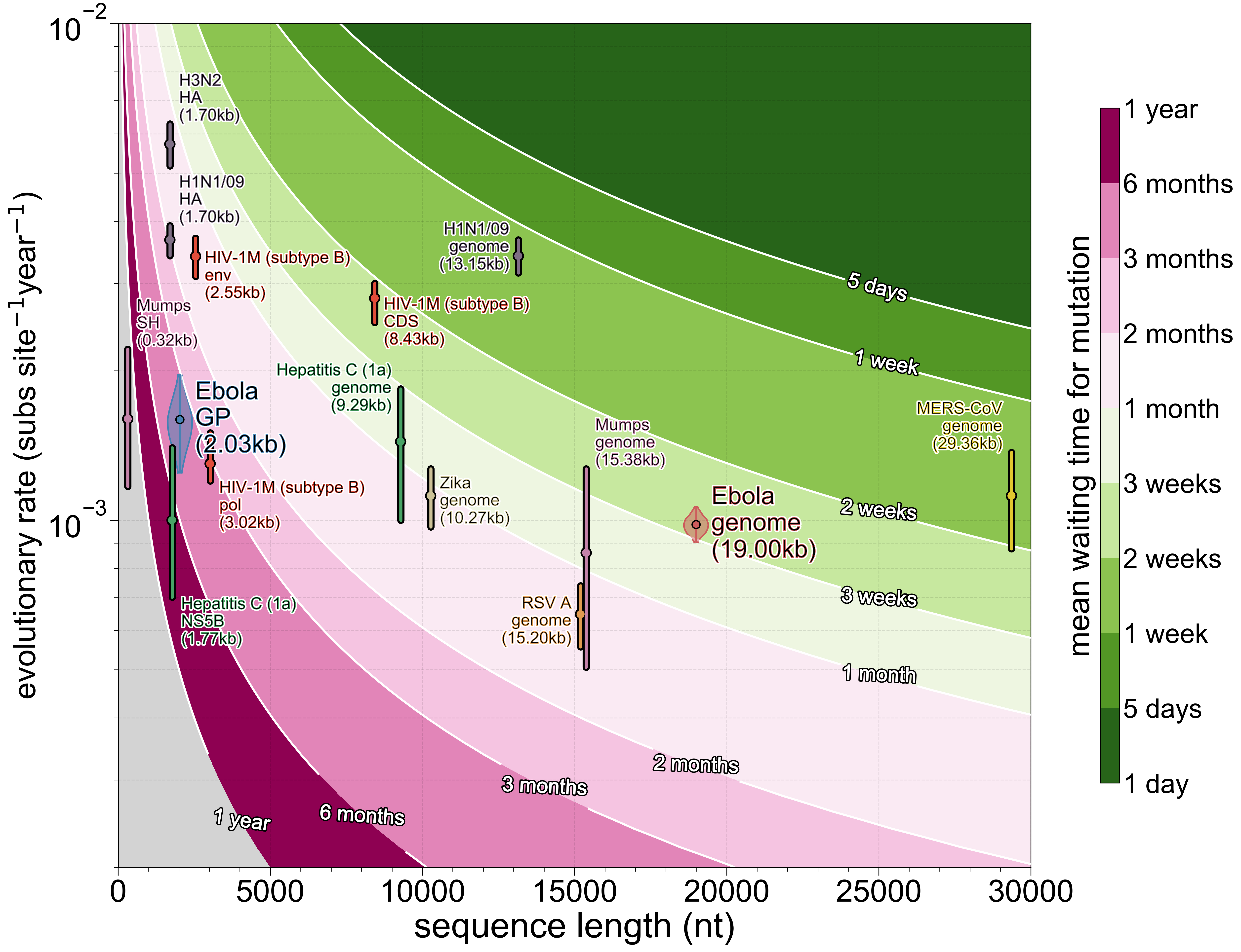
Almost every virus is capped at around one mutation every ~3 weeks and the few things that exceed that threshold, mainly influenza A (very high evolutionary rate and moderate numbers of sites) and MERS-CoV (a very long genome and moderate evolutionary rate), are made more difficult to analyse because both evolve non-clonally to some extent (reassortment and recombination, respectively). In turn this means that processes occurring faster than those timeframes are impossible to encode with any fidelity in viral genomes.

The futility of partial sequences

The evolutionary rate parameter R we’ve been talking about is something that researchers get to pick from a limited range of values, but never fully control. One way of increasing R is to sequence very intensely because it captures circulating deleterious variants that will get purged from the population eventually. You can also find regions of the genome that evolve faster than average, but for a variety of population genetics reasons you’re unlikely to ever encounter a region that will fully compensate the temporal resolution that you lost by not sequencing complete genomes. Let’s come back to our mean waiting time for at least one mutation (1/RL) and express L as Gf (genome length times fraction sequenced), which becomes 1/RGf. Assume that we have identified a single contiguous region comprising 10% of the genome that evolves at a rate twice as fast as the genomic average which sounds sweet! But then keep in mind that whatever’s been lost in G (genome length) because f (fraction that’s sequenced) is reduced needs to be made up for by R (evolutionary rate). In order to maintain the temporal resolution that full genomes allowed the 10% (f=0.1) that we’re sequencing would need to evolve at a rate that’s 1/f higher than the genomic average i.e. 10 times faster. Even for moderate values of f the speed up in R required to maintain the temporal resolution available with complete genomes is excessive - for 40% of the genome (f=0.4) evolutionary rate R needs to be 2.5 times higher (which is still unrealistic for site-wise rate heterogeneity) and by the time you’re sequencing 40% of the genome you might as well be sequencing the remaining 60%.

The lesson here is that more sequences do not always mean more information. If your aim is to know how many cases of something are caused by lineage A or B then sequencing 100 000 sequences that are 100 nt long might be a perfectly valid approach, but you would definitely want to sequence 1000 sequences that are 10 000 nt long if you cared about anything more than just what organism you’re sequencing. Even then there will be a limit, a horizon, to what genomic data can tell you about processes that occur faster than the rate at which genomes are made different by mutations.

Empirical tests

Methods

To demonstrate/test the effect of reducing alignment length on inference we decided to use a traditional machine learning type method of train-test split. We took 1610 Ebola virus genomes (~19,000 nt long) from our earlier study, kept only those that didn’t have too many ambiguous sites and where we knew where (down to 2nd admin level) and when (year-month-day) it had been collected. That still left us with ~900 sequences so we additionally down-sampled this to 600 genomes and picked 60 of those at random which would be our test set. We pretended that we didn’t know when and where those 60 sequences were collected. Then we produced a secondary dataset from the 540 training and 60 testing genome sequences by extracting just the glycoprotein (GP) gene (~2000 nt long). Though a variety of Ebola virus genes had been used as markers in the past GP probably would have been a popular choice before widespread genome sequencing (though subject to primer binding site conservation). At this point we ran the same phylogeographic analyses (generalised linear model, GLM) in BEAST that we used on the complete 1610 genome dataset, only this time it was a dataset of 600 genomes and 600 GP sequences.

Tip date inference

There were two broad aspects of the data we decided to quantify - how well we can infer collection dates and how well the phylogeographic model is performing. The effect of using either genomic or GP sequence data on the ability to infer collection dates ended up being a very persuasive and intuitive figure. It’s very clear that complete genomes are highly informative about when a sequence was collected, with higher precision (narrower confidence intervals) than GP sequences and though the 95% highest posterior density interval for dates encompasses the true date of a sequence more often with GP sequences it’s hardly impressive given how wide those intervals are.

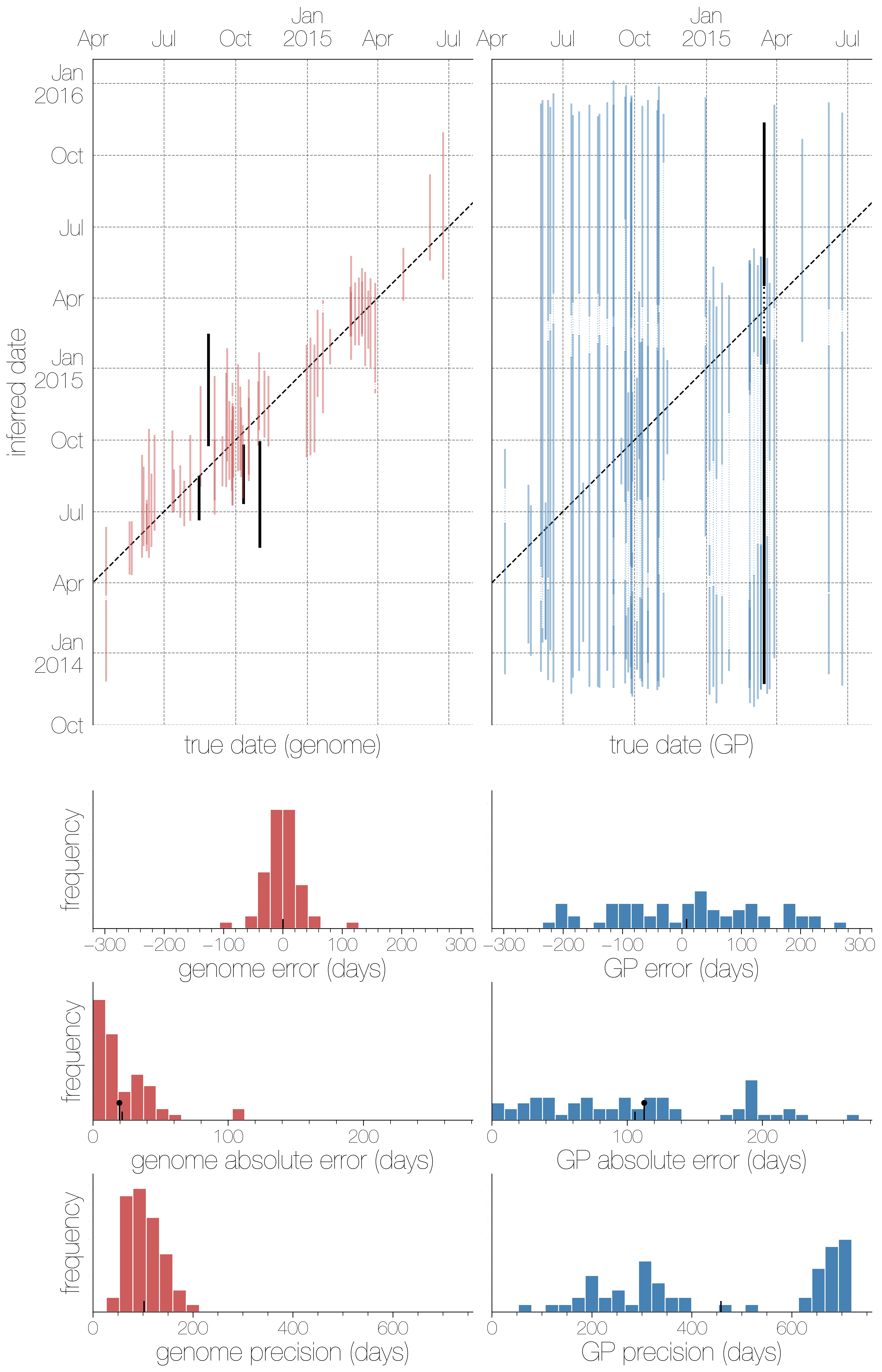
The histograms underneath the scatter plots are (in descending order): signed errors (mean posterior estimate - true date), absolute error (|mean posterior estimate - true date|) and precision (upper confidence bound - lower confidence bound). In every histogram the small black hatch indicates the mean value. The one surprising finding here is that in the third row the hatch indicating the mean and the slightly taller black lollipop are remarkably close. That lollipop is the theoretical expectation from 1/RL. You always expect some error to exist simply because conditioning on a mutation having taken place there will be a distribution of waiting times (and hence dates) for when it could have taken place, but to see empirical results match expectations from such a simplistic model so well was still surprising.

Geographic inference

Inferring the location of masked tips between the two alignment lengths ended up being a bit less clear. Both types of data are a bit bad at informing the model of where the masked tips came from - genomes do slightly better than 50% at guessing the correct location (0.540) and around twice as good as GP sequences (0.286). While tip locations are re-inferred passably the overall history of the epidemic remains surprisingly consistent between both genome and GP sequence data. We suspect that this is driven largely by collection dates and locations of sequences - the epidemic wasn’t everywhere all the time and neither were the sequences. Even before our original publication came out I came across at least one other study that identified a gravity model at work from case data alone.

Even then differences in migration histories explored during MCMC make it very clear that genomes contain sufficient information to exclude a large number of migration histories that are still plausible with GP sequences. The most encouraging finding of all with regards to the migration model is that it’s well-calibrated. What this means is that the model usually proportions its belief to the evidence - it won’t guess strongly in favour of a result if it’s not certain.

What that means for your data

“To consult the statistician after an experiment is finished is often merely to ask him to conduct a post mortem examination. He can perhaps say what the experiment died of.”

RA Fisher (who also argued against tobacco causing lung cancer)

If you’re in a position to generate sequence data for a study think about the process you’re interested in and how fast it’s occurring and then ask yourself if the data you’ll generate will even have a chance of capturing features of the process you’re interested in. There’s no point in sequencing 100 nucleotide fragments of a virus for an outbreak source attribution study because regions that short will experience a mutation on the order of years to a decade, on average. Worse yet it can lead to expected features of the sequence data, e.g. short sequences collected over short periods of time not having any mutations, being confused for phenomena. This has very much been the case for ill-defined and hollow reassurances of “genetic stability” of Ebola virus based on short sequences from outbreaks that lasted months.

Another important consideration is the lifetime of the sequences beyond your study. A genome is a complete whole - you cannot sequence any more of it (usually). What that means is that genomes are trivial to combine across studies, a genome is a genome no matter what study it was sequenced for. This is not necessarily the case for barcode genes of which there can be many and which can be of varying lengths between labs. Recovering a single coherent phylogeny that describes the history of two or more disjoint aligned fragments is impossible without closely related complete genomes or some seriously impressive priors.

Finally, if you won’t sequence complete genomes for the sake of public good but are also into Bayesian methods and about to generate a gigantic dataset in terms of sequence numbers then do it for yourself. It has been exceedingly painful trying to get those effective sample sizes to the arbitrary standard of 200 with the Ebola GP data because MCMC just won’t mix. I remember seeing Chris Whidden present on MCMC exploration of tree space through the subtree prune and regraft (SPR) lens which made it very clear what a waste of CPU cycles the inclusion of identical sequences can be for MCMC. When a lot of sequences have identical backgrounds (i.e. highly polytomic internal nodes as was the case for the Ebola GP data) MCMC will probably accept most topological moves and without appropriate tuning of topological operators (definitely not the case for SPR, NNI and TBR moves) is unlikely to settle down on anything resembling stationarity.

tl;dr

1. Don’t be surprised that your virus phylogeny is a massive polytomy (and therefore as useless as a tree can get) if you sequenced a short gene from infections that are days apart. Mutations (i.e. branch lengths) take time and opportunity to happen. Higher evolutionary rates help with time, longer sequences help with opportunity.

2. Calculating (1/(alignment length * evolutionary rate)) for your sequences is a good proxy for how long it takes for a mutation to crop up in your organism on average. If that number is on the order of years perhaps consider writing a paper about a sequence-based diagnostic method because you certainly don’t have the data for anything phylodynamics-y.

3. Please be considerate to others. No one wants to analyse combined sequences of gene A (lab 1’s favourite) and gene B (lab 2’s favourite) because those data are impossible to combine without closely related complete genomes to bridge the information. No one wants to run MCMC on hundreds of identical sequences either because exploring tree space is hard enough already.

Side note

Academic publishing continues to meet all expectations. The initial submission had to be in the journal’s format. The editorial submission system was broken and my emails about it were ignored for months. After being ignored for months it took the journal minutes to ask for publication fees after accepting the manuscript. Proofs arrived with someone else’s figures. Not all of my comments about proofs were implemented. I’d rate the experience a solid 3/10 and will try avoiding the journal in the future.