Reassortment networks and why I think they’re cool

Why you’re reading this

This blog post will be a bit unusual. Normally I’d like my blog posts to present the “behind the scenes” context for papers that explain the logic of certain decisions whilst also explaining papers casually. This blog post will be very different as I did not play a key role in the paper I’m about to discuss (I’m a co-author though). You may have noticed that on my website I split the papers I’ve been on into “publications” and “contributions”. What I call publications are papers that wouldn’t have materialised or wouldn’t have materialised in their shape had I not been on board. The papers I refer to as contributions are for cases where I wrote some code, made a figure or ran some analysis but wouldn’t feel comfortable calling my own. While Nicola Müller’s new paper on reassortment networks is distinctly a contribution for me I think it has potential to impact the field in profound ways and thus should be popularised more widely.

What is reassortment?

Reassortment and I go way back. If the West African Ebola virus epidemic hadn’t gotten me involved in a bewildering array of papers my first first-author piece of published scientific research would’ve been on reassortment in human influenza B viruses (a topic that deserves its own blog post eventually). Reassortment is a special case of recombination that occurs in viruses whose genomes are split across physically unlinked RNA molecules referred to as segments. If two or more genetically distinct viruses coinfect the same cell the progeny virions coming out of the cell can contain a mixture of segments from different parents. Influenza viruses are perhaps the most widely known examples of segmented viruses, but there are plenty of other examples too (e.g. Partitis, Rotas, Bunyas, etc). In RNA viruses that are positive singled-stranded or double-stranded recombination can occur on top of reassortment, but for the most part everyone analyses segments as independently evolving fragments, so basically like recombination with known breakpoints.

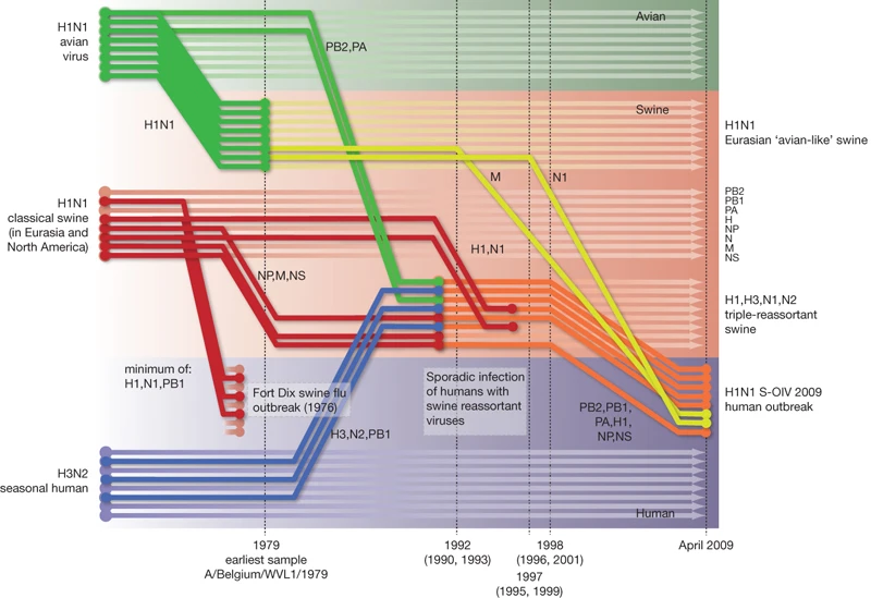
Reassortment is overwhelmingly important for generating pandemic influenza viruses. Most of 20th century pandemics were caused by seasonal human influenza A viruses swapping a couple of their segments for avian influenza A virus counterparts. The segment coding for the surface protein haemagglutinin (HA) would always be swapped out in pandemic viruses, suddenly making them completely new in the eyes of everyone’s immune system. The way we know these things is by building trees of every segment and seeing where each sample falls across the 8 (for influenza A and B) segment phylogenies and reconstructing in our mind’s eye what tree operations could turn one segment’s tree into another. It’s a modestly complicated exercise that needs to happen after every influenza pandemic and it’s quite entertaining. It also leads to cool graphics.

Once we’re done figuring out how a pandemic originated you probably want to shift focus to phylodynamics of the new virus on the human side. Since the virus appears new to population level immunity the virus explodes in numbers, making the viral population quite homogenous during its first sweep. Since there’s not much diversity to speak of and the virus hasn’t had much time to circulate around most people won’t have co-infections, let alone co-infections with genetically distinct strains, few would complain if you ditched the multi-tree approach to sequence analysis and treated the entire genome as a single clonal block. A couple of years later when there’s enough accumulated diversity across segments and the occasional reassortment is when you should go back to using multiple trees to look at our imaginary pandemic influenza virus. In this blog post I will argue that not only is this analysis approach no longer needed but that it is good we don’t.

Overparameterising evolution

In my MERS-CoV recombination paper I made the observation that despite abundant and overwhelming evidence of recombination in MERS-CoV genomes analysing MERS-CoV sequences as either a single clonally evolving block or two blocks split across a statistically significant breakpoint evolving independently on two trees, the former clonal model fit the data much better according to marginal likelihood estimates. The rationalisation then (and now) is that recombination in MERS-CoV is just a light peppering of homoplasies across numerous branches, so adding the extra tree (that’s at least another N*(N-1) parameters to infer) overparameterises the “clonal lite” model of MERS-CoV evolution we postulated and thus a single tree is sufficient to explain the data.

For detectable reassortment to occur in influenza viruses there must be co-infection of a single host not only with genetically distinct viral genomes but co-infection with reassortment-compatible viral lineages. Influenza A and B viruses are far too diverged to reassort naturally and even human-origin inter-subtype influenza A reassortants don’t fare so well. This is a roundabout way of saying that in human influenza co-infection is not the norm - an influenza virus will usually depart a human host with whatever segments it arrived with, perhaps sprinkled with a few new mutations. Each time we add a new segment tree to the analysis we’re introducing at least N*(N-1) parameters in an attempt to accommodate a small number of reticulate branches.

You might remember my previous blogpost or paper where I talked about the rate at which mutations are observed in alignments of different lengths and evolving under different rates. There we chose to quantify the ability of mutations to resolve time by estimating the mean waiting time to a mutation as a function of evolutionary rate R across an alignment with L sites, which ends up being 1/RL. The shorter the mean waiting time to a mutation the more informative the dataset about the passage of time, like stopwatches are more informative than wristwatches because stopwatches have a millisecond hand that wristwatches don’t. It’s nearly guaranteed that best resolution with sequence data is achieved when you analyse full genomes and even then most RNA viruses accumulate mutations on the order of weeks. To maintain the same resolution (mean waiting time to mutation) a shorter alignment needs to evolve at a rate 1/f faster than the full genome where f is the fraction of the genome. You can see the problem already.

If you take the genome-wide evolutionary rate and genome length of the 2009 H1N1 pandemic influenza virus (3.4*10^-3 subs/s/y and 13kb, respectively) you expect the mean waiting time for a mutation to be around 8 days. You can think of this term as the lower bound on the error of a well-calibrated molecular clock model. Unless you’re using some next generation phylogenetics you cannot escape the uncertainty of around 8 days when dealing with a dataset of this length evolving at this evolutionary rate. When you reduce the alignment length by analysing sequence data one segment at a time you’re losing statistical power. Your 8 day uncertainty that you could do nothing about turns to 2 months of uncertainty. The confidence intervals around the timings of your segment tree nodes would increase around 8-fold from the genome-wide tree.

Finally there’s another overlooked problem that only arises in certain analysis setups. If you’re running a molecular clock tree you’re also picking a tree prior. If you choose to give each of your segments an independent tree prior you run into the problem of not having enough sites per segment to be very informative. Linking the tree priors into a single model seems like the right thing to do, but as Nicola found out it’s actually terrible. While introducing extra trees to explain largely clonal data might be overparameterising, treating the then poorly-informed tree nodes as independent data in a coalescent framework ends up double counting the data. If we believe that influenza virus evolution is mostly clonal then coalescences mostly represent whole-genome transmission events. Clusters of coalescences across all of our “independent” loci can only be interpreted as extremely low effective population size by the coalescent. Empirical data agree.

Reassortment networks

Specifying a new statistical model is relatively easy compared to writing code to efficiently explore new parameter spaces with MCMC. Clonal tree operations alone move the tree through some pretty complicated spaces so you can imagine how difficult it must be to write something that efficiently traverses space that has even more dimensions. The data structure that gets sampled during MCMC is a tree that contains tip-like edges that carry the genetic material of some segments to another branch. If you wanted to recover the descent of any given segment you would traverse back from a tip of interest back towards the root unless the branch being traversed contains a reassortment contribution that carried the segment in question, in which case you’d switch your traceback towards the root from where that reassortment edge descended. When visualised reassortment networks are dense with information but ultimately not the easiest to interpret, especially if you want segment-level information.

Visualisation challenges

Visualising reassortment networks as trees with edges of a different kind is relatively easy, but I struggled at first to think of useful things to highlight. Highlighting clonal parts of the tree (i.e. evolution between reassortment events) seemed like a good idea and the first thing I tried was making an exploded tree equivalent where each clonal section of the tree would be offset along the y-axis. Since you’re not seeing it here I didn’t think it worked very well. Networks are messy to begin with and moving away from a tree-like layout with reassortment edges criss-crossing just seemed to strain the eye too much. What I did instead is colouring branches a new colour after a reassortment event using a non-intrusive cycle of sequential colours (like this but less vivid) which I thought did the job relatively well:

The next challenge was reassortment edges. In Nicola’s paper I chose to display these as lines that represent each reassorting segment as a line of a particular colour:

I think that works fine, though I’ve also experimented with highlighting segments with a row of binary boxes (bottom):

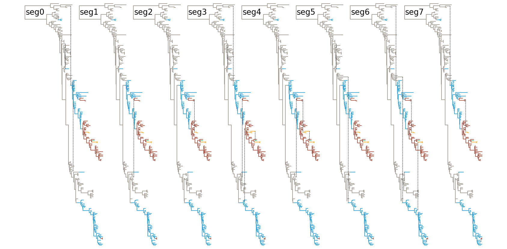
And finally one can continue sticking with multiple trees, but highlighting the clonal path of each segment:

Obviously, I’m still trying to find better ways of visualising these and I’m very open to suggestions.

The potential

So far I’ve been talking about how reassortment networks are better at utilising information and how annoying it is to plot them in a satisfactory way. I now invite you to imagine the possibilities of what is possible.

More power

In order for reassortment to occur two viral genomes must find themselves in the same cell. If two viral genomes are in the same cell you can be sure they’re in the same geographic location too, so if you were able to run something like your typical discrete trait analysis on top of a reassortment network you’d be leveraging the same levels of information that we gained access to in molecular clock analyses. We’re talking more power to infer timings and more power to infer state transition rates, so what’s not to love?

Reassortment distance

In my 2014 influenza B reassortment paper I used a metric called 𝛿TMRCA. It was the difference in most recent common ancestor dates for the same pair of tips in two different segment trees. The idea is that if the two numbers are really different the more recent TMRCA will correspond to a reassortment (because one of the lineage’s evolutionary history was overwritten by an incoming lineage) and the older TMRCA is a genuine common ancestor (though it could be another reassortment event too). That distance is meant to represent the amount of independent evolution that has occurred between two segments since they were part of the same genome until they encountered each other again in a reassortant genome. Alternatively you can think of it as your reassortment signal - genomes reassorting after diverging for a month are likely to be identical (and thus reassortment undetectable), but segments reassorting between genomic backgrounds that have been diverging for decades would be very easy to spot. This is in fact what Nicola and co showed in their Figure 1C:

Depending on the limitations of the system you could look at the rate at which different parts of the same viral genome diverge epistatically, i.e. the rise of Dobzhansky-Muller incompatibility. I described an example of this type of incompatibility in my influenza B reassortment paper (later confirmed in cell culture) and Villa & Lässig described this in much finer detail for influenza A viruses.

Co-reassortment

Obviously the other thing that you can look into using Nicola and co’s method is co-reassorting segments. We convinced ourselves that co-reassorting PB1-PB2-HA segments in influenza B were the result of post-reassortment selection on hybrid PB1-PB2-HA segment constellations, but another possibility is that co-reassortments occurs via some peculiarity of the segment packaging mechanism. Barring intensive analyses of gigantic sequence datasets or exhaustive cell culture experiments there’s no easy way of seeing if segments are co-reassorting. For something with 8 segments like influenza A and B there are 254 different kinds of reassortants (2^8-2, where you pick whether a given segment was reassorted or not minus where all segments are derived entirely from one or the other parent) that can be produced from a co-infection. To establish statistically significant differences in observation rates between particular segment combinations you clearly need very high numbers of reassortments. While this doesn’t apply to specific hypotheses (e.g. particular labeled lineages do not reassort across a defined number of potential reassortment opportunities) it makes exploratory analyses unfeasible. As such, despite my optimism about reassortment networks in general I believe this one is an inherent limitation of the data that no method can solve easily.

Unforeseen cases

I can’t help but approach reassortment and what I’d like to learn about the process with the personal biases that brought me to the topic in the first place. So if I have missed a potential avenue of research do tell me so I can update this section of the blog post!

Final thoughts

We may be in the middle of a coronavirus pandemic in the year 2020 but let’s not forget the other F word that comes to mind when we talk about pandemics - flu. When the next influenza pandemic hits I’m hoping that Nicola’s reassortment network model will have been picked up, improved upon and deployed widely, simply because it’s the only method that maximises sequence data use and reduces the amount of data post-processing in segmented datasets. To summarise, if you have all segments of a measurably evolving virus and you want the best possible segment trees under the constant population size coalescent tree prior you can’t do any better right now than reassortment networks™.